Mastering DP-500: Synapse Analytics Dedicated SQL Pools – Everything you need to know!

DP-500 Table of contents

In the previous article, you’ve learned how to leverage the Serverless SQL pool to query the data stored within various file types in your Azure Data Lake. We’ll stay in the SQL world again, now examining various concepts and techniques related to a Dedicated SQL pool in Azure Synapse Analytics.

A short disclaimer: the official exam sub-topic is called: querying the data from the Dedicated SQL pool. But, in the end, it’s just a SQL, so I’ll not teach you how to write T-SQL code, nor provide specific T-SQL “how-to” solutions…Therefore, if you are looking to learn and understand SQL, this article is not for you…

In my opinion, it’s way more important to understand different concepts and techniques that distinguish a Dedicated SQL pool from the traditional SQL Server, and how to leverage these concepts and techniques in real-life scenarios. Obviously, learning this stuff will definitely help you to get ready for the DP-500 exam, but what’s even more critical, will give you a broad understanding of the “traditional data warehouse” part of the Azure Synapse Analytics platform.

Back to basics

But, let’s first back to basics, and briefly explain the key components of the data warehousing workloads.

When you’re designing a traditional data warehouse, there are two main types of tables that you’d create:

• Dimension tables describe various business entities, such as customers, products, time, and so on. The way I like to think about dimension tables is: they should answer the business questions starting with W:
  • What did we sell? Product X
  • Where did we sell? In the USA, for example?
  • Whom did we sell? To a customer ABC
  • Who did sell? Employee XYZ?
  • When did we sell? In the 1st quarter of 2022, for example
• Fact tables answer the question: How much? How many sales did we have? In addition, fact tables may contain measurements or events that occurred – for example, stock balances, measured temperatures, and so on.

Unlike in online transaction processing systems, or OLTP abbreviated, where the data model is denormalized to support fast INSERT, UPDATE and DELETE operations, in online analytical processing systems, or OLAP, it’s not uncommon to have redundant data in dimension tables, thus reducing the number of joins when running analytical queries, where the main operation with the data is READ.

The physical implementation of the tables

Fine, now that you understand the two main table types from the conceptual perspective, let’s focus on explaining how the tables are physically implemented within the Azure Synapse Analytics Dedicated SQL pool.

When it comes to data persistency, there are three main table types:

• Regular table, which stores the data in Azure Storage as part of a Dedicated SQL pool. Data is persisted in the storage regardless if the session is open or not
• Temporary table uses local storage to store the data temporarily, only while the session is opened. The main reason for using temporary tables is to prevent users outside of the session to see the temporary results, but also to speed up the development process by storing the intermediate results in local instead of remote storage

• External table, similar to the one that we examined in the previous article, points to the data stored in Azure Data Lake or blob storage. External tables may come in handy when loading the data into the Dedicated SQL pool

Partition elimination

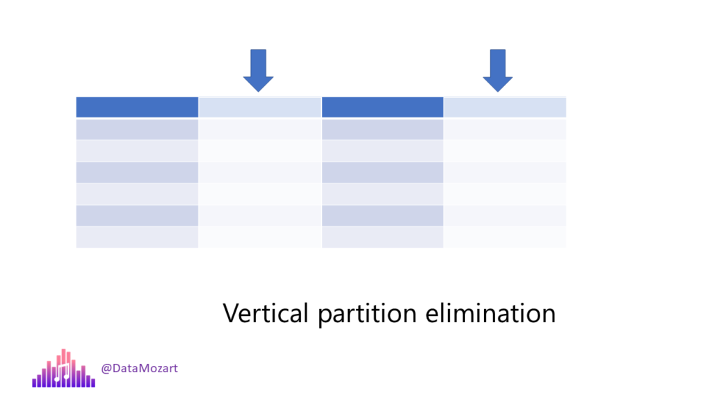
You’ve already learned in the previous article about the concept of partition pruning, or partition elimination. Remember, the Serverless SQL engine was able to skip the scanning of unnecessary data. Depending on the file type, it was possible to take advantage of horizontal and vertical partition pruning.

A similar approach is also available in the Dedicated SQL pool. The most common scenario is to partition the data on the date column. Obviously, depending on the amount of data, you may decide to partition on year, month, or day level. The overall query performance can be significantly improved by applying an appropriate partitioning strategy. However, be mindful when creating partitions, as sometimes too many partitions can downgrade the query performance.

There is no single golden number of partitions that you should create – essentially, it depends on your data, and the number of partitions that need to be loaded in parallel. Although there is no single golden number of partitions for the table, in reality, we’re usually talking about tens or hundreds of partitions, but definitely not thousands…

If you’re partitioning the data in clustered columnstore table, you should think about the number of rows that will go in each partition. To get the optimal compression rate, every distribution and partition should contain at least 1 million rows. Also, keep in mind that the Dedicated SQL pool’s architecture is based on massively parallel processing, which means that even before you create your partitions, each table is already split into 60 distributions.

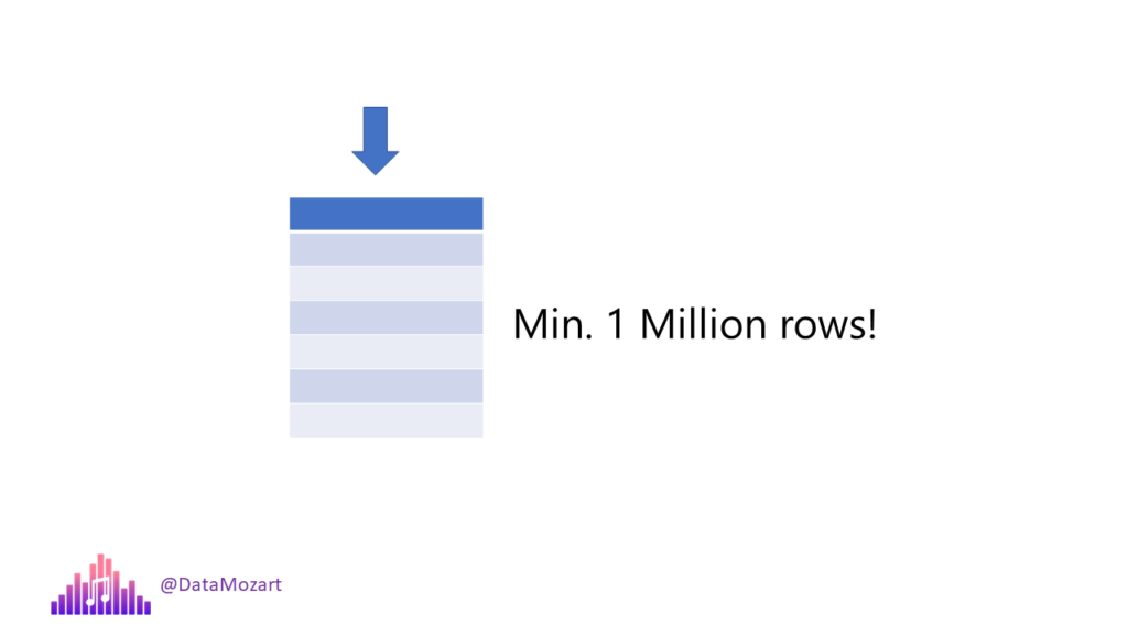
Table partitioning can also bring multiple benefits to the data loading process. The final thing to be aware of regarding partitioning is that you can apply partitioning only on one column.

Indexing and statistics

Another two important features for increasing the efficiency of the Dedicated SQL pool workloads are columnstore indexes and statistics.

You may be already familiar with columnstore indexes from the good old days of SQL Server. Now, in the Dedicated SQL pool, your table is by default stored as a clustered columnstore index, which enables a high compression rate and fast performance for analytic queries. Aside from clustered columnstore index, you can choose between clustered index or heap, where heap may be the optimal choice in the data loading process, for creating staging tables.

Last, but not least, statistics help the engine to generate the optimal query execution plan. It’s of paramount importance for columns used in query joins, WHERE, GROUP BY, and ORDER BY clauses. Please keep in mind that while creating statistics happens automatically, updating statistics requires action from your side. So, it’s a recommended practice that you perform an update statistics operation once the data loading process is completed.

(Un)supported table features

I’ll wrap this tables’ story by compounding the list of all unsupported table features in the Dedicated SQL. If you’re coming from traditional SQL Server background, you may find missing some of them quite intimidating.

There is no possibility to check foreign key constraints in the Dedicated SQL pool. So, the responsibility for ensuring the data integrity is on your side, not the database itself. Other important unsupported features are computed columns, unique indexes, and triggers.

Table distribution options

One of the fundamental features of the Dedicated SQL pool is the possibility to define the way your data is going to be stored. As you might already know, a Dedicated SQL pool works as a distributed system, which means that you can store and process the data across multiple nodes. To put it simple, this assumes that the parts of your table, or the whole table, will spread across multiple locations.

A dedicated SQL pool supports three options for data distribution. It’s a crucial task to understand the way these distribution options work, as this may have a huge impact on the overall workload performance.

Round-robin is a default option. It randomly distributes table rows evenly across all distributions. The key advantage of this method is fast data loading, while the most noticeable downside is the fact that retrieving the data from Round-robin tables could require more data movement between the nodes, compared to other distribution options. Also, join operation on round-robin tables may be inefficient, because the data has to be reshuffled. To conclude, Round-robin tables are great for data loading and bad for querying, especially for queries that include joins

Hash-distributed table operates completely differently. Based on the value in the column which is selected for distribution, a certain row will be allocated to a specific distribution. This option enables high-level performance for queries over large tables, such as giant fact tables with millions or even billions of rows. The key ingredient for this concept to work is the deterministic hash algorithm that assigns each row to one distribution.

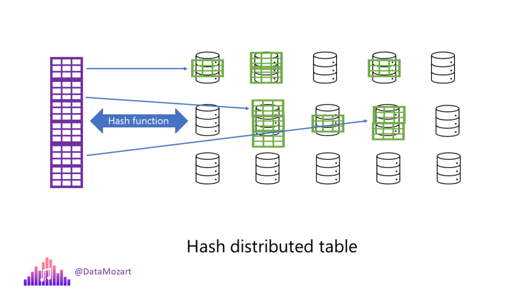
It’s important to keep in mind that each row belongs to one distribution. Unlike in Round-robin tables, where rows will be evenly distributed across multiple nodes, with Hash tables number of rows per distribution may vary significantly, which means that, depending on the data in the hash column, you may have tables with very different sizes between different nodes.

To wrap it up, hash tables are great for reading the data from large fact tables in a star schema, including joins and aggregations. You should consider using hash tables when your table size is greater than 2 GBs.

One of the crucial decisions you need to make is choosing the column for distribution. When choosing the distribution column, you should take into consideration the number of distinct values in the column, data skew, and estimation of the type of the most frequently run queries. Keep in mind that once you’ve chosen the distribution column, you can’t change it, unless you recreate the whole table. To get the most out of parallel processing performance, your distribution column should check a few boxes:

• Many unique values – all rows with the same value will be allocated to the same distribution. Since there are 60 distributions in total, if you have let’s say, 10 unique values, you will get many distributions with 0 values assigned, so there is no benefit of parallel query processing
• Not a date column – as we’ve already learned that rows with the same values will be assigned to the same distribution, imagine the situation where all your users are querying the data from the last 7 days. In this case, only 7 distributions will perform the whole processing work, instead of spreading that work across 60 nodes
• No NULLs, or contains just a few NULLs – similar to previous scenarios, imagine that you have a column containing NULL values only. This will allocate all the rows to a single node, so there is no parallel processing at all!

The third option for data distribution is the replicated table. This one is the simplest to explain: a replicated table stores the full copy of the table on every single node. Since there is no data movement between the nodes, the queries run fast.

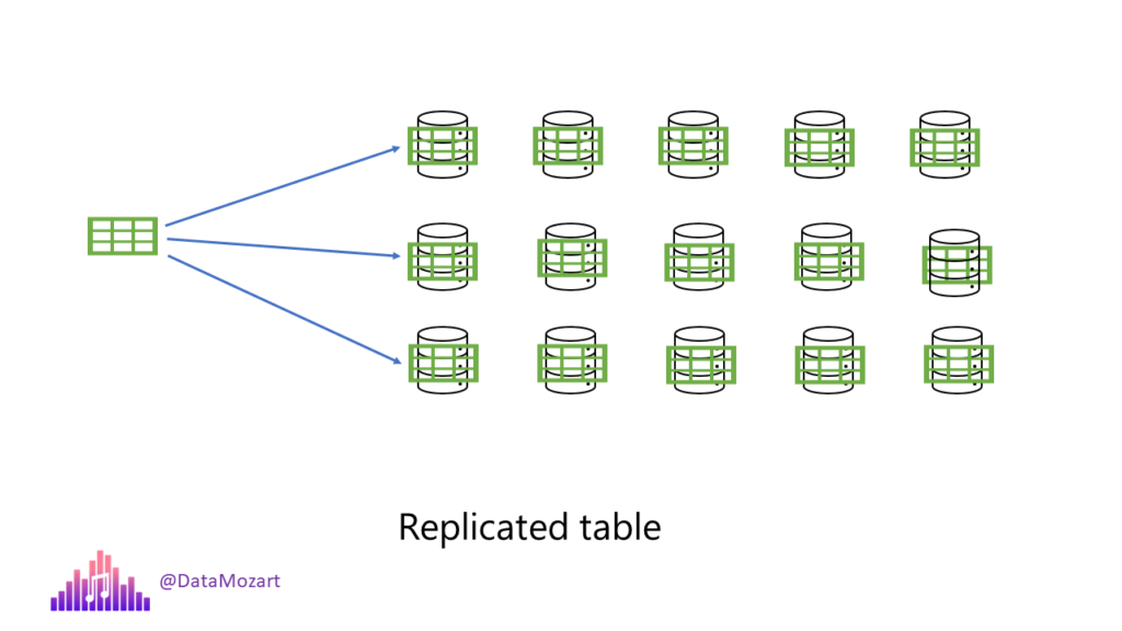
I hear you, I hear you: Nikola, if the queries run fast, why don’t we simply always use replicated tables? That’s a fair question, so let me quickly answer it. By creating replication tables, we are basically creating redundant data. Each of these replicas has its own memory footprint and requires additional storage. This means it’s not the most optimal solution for large fact tables.

In a real-life world, this distribution option mostly suits dimension tables from the star schema. Although there is no hard limit on the table size you should replicate, the recommended practice is to use this option for tables smaller than 2 GBs, regardless of the number of rows.

While replicated tables offer fast query performance, they are not the preferred option for DML operations, such as insert, update and delete, because each of these operations requires a rebuilding of the entire replicated table.

Performance optimization tips and techniques

As you may know, a Dedicated SQL pool provides a separation of the storage and compute power. Consequentially, you can independently scale compute power from storage and vice versa.

Let’s kick it off by explaining how scaling out works with compute layer. When you provision a Dedicated SQL pool, you get exactly 60 distributions provided. However, the exact compute power depends on the number of data warehouse units you select.

Wait, what on Earth is now a data warehouse unit? Well, this is a unit that represents the combination of CPU, memory, and IO. The greater the number of a data warehouse unit, the more powerful it will be.

Based on the number of compute nodes, the number of distributions may also vary, as you may see in the following table:

As you may assume, the more compute nodes you have available, the higher performance you should achieve.

Now, the fair question would be:

How many DWUs do I need?

And, I’ll immediately give you a very straightforward answer: it depends😊

The recommended practice is to start with a smaller configuration, for example, DW200, and then, based on the insights obtained from monitoring your workloads, define if and when to increase the number of data warehouse units.

Scaling out the data warehouse will have an impact in the following areas:

• Performance improvement for table scans, aggregations, and CREATE TABLE AS SELECT operations
• Enable more data readers and data writers
• Increase the number of concurrent queries and concurrent slots

As you may expect, there is no single golden advice on when to scale out DWUs. However, you may want to consider it during peak business hours – let’s say that every Monday, many users run a complex report based on the data stored in the Dedicated SQL pool. In order to avoid concurrency issues, it’s a good idea to increase the number of resources during that period. Afterward, you can easily scale the number down again.

Also, if you are performing a heavy data loading workload or some complex transformation, scaling out the capacity will help you to complete these operations faster and have your data available sooner.

However, don’t think that moving this DWU slider all the way to the right will auto-magically resolve all your performance issues. In case you notice that there is no performance improvement, or no significant improvement, your problem probably lies somewhere else – and maybe you should consider checking table distribution options.

Query performance tuning

The first solution is the usage of the Materialized views. Unlike a “regular” view, which computes results every time your query targets it, materialized views, as their name suggests, materialize the data in the Dedicated pool, same as for the regular table. Since the results are already pre-computed and stored, queries targeting materialized views usually perform better compared to ones pointing to standard views.

Not just that implementing materialized views will reduce the time for executing complex queries, what’s even better, you can distribute the data from the materialized view differently than the data from the original underlying tables, which provides even more opportunities for optimization.

However, as with every powerful feature, this one also comes with some tradeoffs. In this case, the biggest one is the tradeoff between query performance and additional costs. Don’t forget that materialized views persist the data in the storage layer, while there are also related costs for maintaining these views.

Indexing is another very powerful technique for optimizing queries. Assuming that you are using a clustered columnstore index for the table, by default, data in the index will not be ordered. There’s nothing inherently wrong with this approach, because with a high compression rate and metadata stored on each rowgroup segment, using a default non-ordered clustered columnstore index will still work well.

However, it may happen that there are overlapping ranges of values in multiple segments, so when the engine scans the data, more segments will be included, thus more time and resources required to complete the query.

On the flip side, when you include an order clause in the clustered columnstore index, the engine will sort the data before it’s compressed into segments, which decreases the number of overlapping values in segments.

Same as in the previous case with materialized views, there is also a tradeoff with ordered vs non-ordered clustered columnstore index. The data loading process will be slower for the ordered index, but the query performance will be better at the same time.

Last, but not least, a Dedicated SQL pool enables you to leverage the result set caching feature to improve the performance of the queries. Once you turn on this feature, a Dedicated SQL will automatically cache all the queries run on that specific database.

What’s the benefit of doing this, you might ask? Well, by storing the query result, every subsequent matching query, may be served from the cache memory. This means, no repeating computation, no occupying concurrency slots, and the query will not be part of the provisioned concurrency limit.

There are certain limitations regarding what queries can be cached, most noticeable, queries that use user-defined functions, or queries that return more than 10 GBs of data. Also, if there were changes in the underlying schemas or tables that are part of the cached result set, the subsequent query will not be served from the cache.

The cache is automatically managed by a Dedicated SQL pool. If it happens that the cached result set was not reused within the next 48 hours, it will be removed from the cache. In addition, keep in mind that there is a maximum result set cache size of 1 TB per database.

Finally, once you’re done querying a Dedicated SQL pool, don’t forget to pause your compute layer, in order to avoid unnecessary costs.

Conclusion

Although a Dedicated SQL pool from many perspectives resembles a traditional SQL Server, the underlying architecture (Massively Parallel Processing) is completely different, which implies that there are certain concepts and techniques that are exclusively applicable to a Dedicated SQL pool.

Knowing in which scenarios to use which table distribution option, or when to scale out your relational data workloads, are some of the key considerations that can make your Azure Synapse Analytics project a success or failure.

Thanks for reading!

Last Updated on January 20, 2023 by Nikola