Mastering DP-500: Synapse Serverless SQL and file types - the ultimate guide!

DP-500 Table of contents

In the previous article of the series, we explained the difference between the two SQL-flavored pools in Azure Synapse Analytics, and, what’s even more important, in which scenario it makes sense to use each of them. By sharing a list of the best practices when working with a Serverless SQL pool, we also scratched the surface of the next very important topic – dealing with various file types!

The purpose of this article is to provide you with a better understanding of what is happening behind the scenes once you run the T-SQL query in Serverless SQL, using either Synapse Studio, or some of the well-known client tools, such as SSMS or Azure Data Studio. It should also give you a hint about the difference in performance and costs, based on the file type you’re dealing with.

CSV files

To put the discussion in the proper context, I’ve prepared two files that contain exactly the same data (it’s a well-known Yellow Taxi public dataset) – once stored as a CSV file, while the other is in parquet format.

Let’s quickly run the first query and check what’s happening in the background:

SELECT 
     *
FROM
	OPENROWSET(
		BULK'https://nikolaiadls.dfs.core.windows.net/nikolaiadlsfilesys/Data/yellow_tripdata_2019-01.csv',
		FORMAT='CSV',
		PARSER_VERSION='2.0',
        HEADER_ROW = TRUE
    )
	as baseQuery

Before I show you the results and metrics behind this query, let’s just quickly iterate over the key parameters of the query: I’m returning all the columns from the CSV file that is stored within my ADLS (it’s the data about yellow taxi rides in January 2019). Within the OPENROWSET function, I specified the file format (CSV), and parser version (2.0 is recommended). The last argument instructs the engine to treat the first row as a header for my columns.

This query returned approximately 7.6 million records, and this is the amount of the data processed (we’ll come back later to explain what counts in the amount of processed data):

Cool! We now have our first benchmark to compare with other query variations.

The next thing I want to try is returning only top 100 rows from this dataset. Let’s imagine that my goal is to quickly understand what’s in there, before I decide how to proceed:

SELECT 
    TOP 100 *
FROM
	OPENROWSET(
		BULK'https://nikolaiadls.dfs.core.windows.net/nikolaiadlsfilesys/Data/yellow_tripdata_2019-01.csv',
		FORMAT='CSV',
		PARSER_VERSION='2.0',
        HEADER_ROW = TRUE
    )
	as baseQuery

And, now the numbers look different:

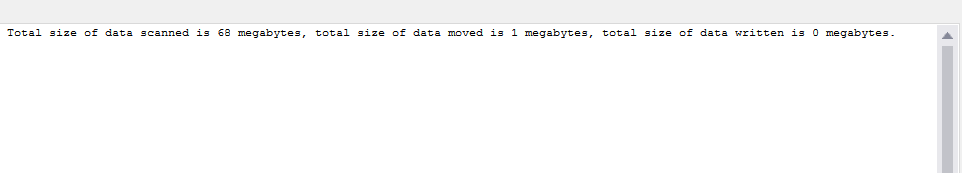
It appears that the engine is capable of eliminating certain portions of data, which is great!

Let’s now examine what happens if we want to retrieve the data only from 3 columns:

 SELECT 
     VendorID
    ,cast(tpep_pickup_datetime as DATE) tpep_pickup_datetime
    ,total_amount totalAmount 
FROM
  OPENROWSET(
    BULK'https://nikolaiadls.dfs.core.windows.net/nikolaiadlsfilesys/Data/yellow_tripdata_2019-01.csv',
    FORMAT='CSV',
    PARSER_VERSION='2.0',
    HEADER_ROW = TRUE
    ) 
WITH(
        VendorID INT,
        tpep_pickup_datetime DATETIME2,
        total_amount DECIMAL(10,2)
    )
	as baseQuery

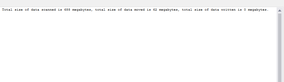
Wait, what?! No, I haven’t posted the original query results by mistake, although the numbers for data scanned are exactly the same! This brings us to a key takeaway when dealing with CSV files:

CSV: No vertical partitioning is possible, whereas horizontal partitioning occurs!

Let’s briefly explain the above conclusion. No matter if you are retrieving 3 or 50 columns, the amount of scanned data is the same. Because the columns are not physically separated, in both cases the engine has to scan the whole file. On the flip side, the number of rows you’re returning DOES matter, because you saw the difference in numbers when we retrieved the top 100 rows vs the whole 7.6 million table.

Schema inference challenges

One more thing before we proceed to query parquet files. You may have noticed that I’ve used the WITH clause in the second code snippet – by using WITH, I can explicitly set the data type for the certain column(s), thus avoiding challenges caused by the schema inference feature.

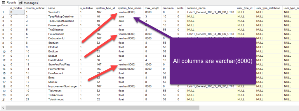
Built-in schema inference enables you to quickly query the data in the data lake without knowing underlying schemas and data types. However, this handy feature comes with a cost – and the cost is that inferred data types are sometimes much larger than the actual data types! For example, parquet files don’t contain metadata about maximum character column length, and inferred data type is always varchar(8000)!

Therefore, before doing “serious” things with Serverless SQL, I suggest you running the system stored procedure sp_describe_first_result_set, which will return all the data types from the file:

EXEC sp_describe_first_result_set N'
	SELECT 
        VendorID
        ,CAST(TpepPickupDatetime AS DATE) TpepPickupDatetime
		,CAST(TpepDropoffDatetime AS DATE) TpepDropoffDatetime
        ,PassengerCount
        ,TripDistance
        ,PuLocationId
        ,DoLocationId
        ,StartLon
        ,StartLat
        ,EndLon
        ,EndLat
        ,RateCodeId
        ,StoreAndFwdFlag
        ,PaymentType
        ,FareAmount
        ,Extra
        ,MtaTax
        ,ImprovementSurcharge
        ,TipAmount
        ,TollsAmount
        ,TotalAmount TotalAmount
FROM  
    OPENROWSET(
        BULK ''puYear=*/puMonth=*/*.snappy.parquet'',
        DATA_SOURCE = ''YellowTaxi'',
        FORMAT=''PARQUET''
    )nyc
WHERE
    nyc.filepath(1) = 2019
    AND nyc.filepath(2) IN (2)'

Based on the information obtained from running this stored procedure, you may decide to adjust the data types for specific column(s).

Parquet files

While discussing the best practices when working with a Serverless SQL pool, we’ve already mentioned that parquet files should be used whenever possible. You’ll soon understand why…

There are numerous advantages of using parquet files, so let’s list just a few of them:

Parquet format compresses the data and this consequentially leads to a smaller memory footprint of these files, compared to CSV
Parquet is a columnar format, and in many ways resembles Columnstore indexes in relational databases. Because of that, the Serverless SQL engine can skip unnecessary columns when reading data from Parquet files, which is not the case with CSV. This will directly affect not just the time and resources needed for processing the query, but will also reduce the cost of that query. With parquet format, the engine also takes advantage of row elimination, as greatly explained in this video from the Synapse product team

Let’s go back to SSMS and run exactly the same queries, over exactly the same amount of data, but this time stored in parquet format:

SELECT 
        *
FROM  
    OPENROWSET(
        BULK 'puYear=*/puMonth=*/*.snappy.parquet',
        DATA_SOURCE = 'YellowTaxi',
        FORMAT='PARQUET'
    )nyc
WHERE
    nyc.filepath(1) = 2019
    AND nyc.filepath(2) IN (1)

As you see, the amount of data scanned is significantly lower compared to the same dataset in the CSV file, although the amount of data moved is greater in this case.

With the top 100 clause included, the numbers are 20 MB (scanned) and 1 MB (moved).

Let’s check the metrics once we retrieve only 3 columns and by handling schema inference:

	SELECT 
        CAST(vendorID AS INT) AS vendorID
		,tpepPickupDateTime
		,totalAmount
	FROM  
		OPENROWSET(
		 BULK 'puYear=*/puMonth=*/*.snappy.parquet',
		 DATA_SOURCE = 'YellowTaxi',
		 FORMAT='PARQUET'
	 )
	 WITH(
		vendorID VARCHAR(3),
		tpepPickupDateTime DATETIME2,
                totalAmount FLOAT
		)
	 nyc
	 WHERE nyc.filepath(1) = 2019
		  AND nyc.filepath(2) IN (1)

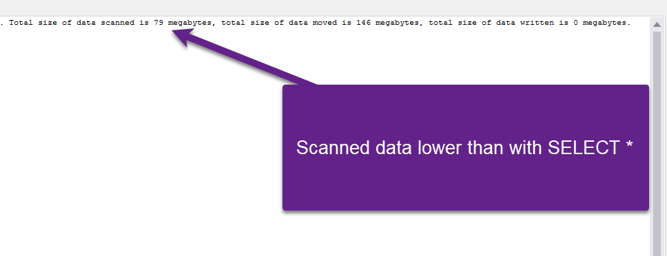
Unlike in the “CSV case”, where the engine scanned exactly the same amount of data in both scenarios (all vs specific columns), with parquet we see that numbers are lower when we’re returning a set of columns instead of all.

This brings us to an important takeaway when dealing with parquet files:

Parquet: Both vertical and horizontal partitioning is possible!

Show me the money! How much do your queries cost?

Before we proceed to delta files, I promised the explanation about the various numbers displayed when you run the query. This is especially important, because, in the end, this shows the “cost” of the query (by the way, we’re talking about real costs, real $$$).

Microsoft boldly says that you will be charged for the amount of data processed. But, let’s dig deep and check what counts for the amount of data processed:

Amount of read data – here, you should count the data itself, but also related metadata for formats that contain metadata, like parquet

Amount of moved data – when you run the query, it’s split into smaller chunks and sent to multiple compute nodes for execution. While the query runs, data is being transferred between the nodes, and these intermediate results are something you should be aware of, same as data transfer to the endpoint, in an uncompressed format. In reality, this number will differ if you run something like: SELECT * from the file that contains 30 columns, from the case when you are selecting only a few columns

Amount of written data to data lake. This applies in those scenarios when you use CETAS to export query results to a parquet file that’s going to be stored in a data lake

So, when you sum up these three items, you are getting the total amount of data processed.

Statistics – as in regular SQL databases, statistics help the engine to come up with the optimal execution plan. Statistics in a Serverless SQL pool can be created manually, or automatically. In both cases, there is a separate query running to return the column on which statistics is built. And, this query also has some amount of data processed

One important remark here is: with Parquet files, when you create statistics, only the relevant column is read from the file. On the other hand, with CSV files, the whole file needs to be read and parsed in order to create statistics for a single column.

Currently, pricing starts from 5 $ for 1 TB of processed data. Also, keep in mind that the minimum chargeable amount per query is 10 MB. So, even though you sometimes have a query that processed less than 10 MB of data, you will be charged as this minimum threshold was reached.

Leveraging FILENAME and FILEPATH function to reduce the queries

There are two functions that you should use to reduce the amount of data that needs to be read from the files.

The FILENAME function returns the file name and can be leveraged within the WHERE clause of the T-SQL query to limit the scanning operation to a certain file or files:

SELECT
    base.filename() AS [filename]
    ,COUNT_BIG(*) AS [rows]
FROM OPENROWSET(
        BULK'https://nikolaiadls.dfs.core.windows.net/nikolaiadlsfilesys/Data/yellow_tripdata_2019-*.csv',
        FORMAT='CSV',
        PARSER_VERSION='2.0',
        HEADER_ROW = TRUE) 
        WITH (C1 varchar(200) ) AS [base]
WHERE
    base.filename() IN ('yellow_tripdata_2019-01.csv', 'yellow_tripdata_2019-02.csv', 'yellow_tripdata_2019-03.csv')
GROUP BY
    base.filename()
ORDER BY
    [filename];

This query will target only these three files whose names we explicitly specified in the FILENAME function.

FILEPATH function works in a similar way, but instead of the file name, it returns a full or partial file path. In the following example, you can see how I’ve swapped asterisk symbols with explicit values, thus instructing the engine to look only for the data for January 2019:

SELECT 
        CAST(vendorID AS INT) AS vendorID
		,tpepPickupDateTime
		,totalAmount
	FROM  
		OPENROWSET(
		 BULK 'puYear=*/puMonth=*/*.snappy.parquet',
		 DATA_SOURCE = 'YellowTaxi',
		 FORMAT='PARQUET'
	 )
	 WITH(
		vendorID VARCHAR(3),
		tpepPickupDateTime DATETIME2,
                totalAmount FLOAT
		)
	 nyc
	 WHERE nyc.filepath(1) = 2019
		  AND nyc.filepath(2) IN (1)

Delta Lake files

The possibility to read Delta format using T-SQL is one of the newer features in the Serverless SQL pool. Essentially, Delta lake is an architecture that provides many capabilities of the traditional relational databases (namely, ACID properties) to Apache Spark and big data workloads. You can leverage the Serverless SQL pool to read the Delta files produced by any system, for example, Apache Spark or Azure Databricks.

Queries work very similar to the parquet format (in fact, Delta is based on the parquet format), including partition elimination, usage of FILEPATH and FILENAME functions, etc, so I’ll not go deep into the details again.

The main difference between Delta and parquet is that Delta keeps a transaction log (think of SCD scenarios, or point-in-time analysis). DISCLAIMER: These are general capabilities of Delta files, not necessarily available in synergy with Serverless SQL (as explained in the next paragraph).

Another important thing that I’d like to emphasize, and which is greatly explained in this blog from Andy Cutler, is that Delta has the capability to evolve the schema based on new source attributes, so the Serverless SQL pool can natively read from the changed files.

However, there are certain limitations when it comes to reading Delta files using the Serverless SQL pool: for example, point-in-time analysis is not available at this moment, as Serverless SQL will retrieve only the current values.

As Serverless SQL in use cases with Delta format is still a work-in-progress, I suggest you regularly check all the known limitations on Microsoft’s official Docs site.

Conclusion

There are many options for querying the files from your Azure Data Lake storage, using the Serverless SQL pool in Synapse Analytics. The key feature of Serverless SQL is that you can leverage a familiar T-SQL syntax to read the data from various file types, such as CSV, JSON, parquet, or Delta.

However, it’s often not enough to simply know what are the limitations when it comes to a set of supported T-SQL features, but also what are the strengths and weaknesses of the file types that store your data.

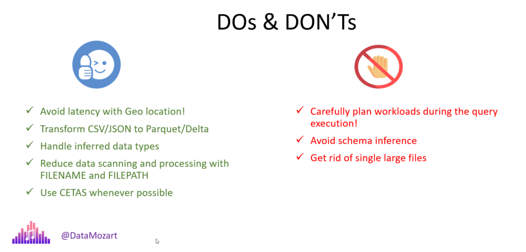
Here is the general list of DOs and DON’Ts for querying files using a Serverless SQL pool: