

This blog post is part of the “Data Modeling” series, created together with my friend and well-known Power BI expert – Tom Martens
Table of contents
- PRELUDE TO DATA MODELING WITH POWER BI
- THE POWER BI DATA MODEL
- Tables, columns and some things related
- Concept of extended tables
- Calculated columns and measures
- The danger of the one-table solution
- Cardinality – your majesty!
- RELATIONSHIPS
- The benefits of strong relationships
- Circular dependencies
- Role-playing dimensions
- Bi-directional relationships
- PARENT-CHILD HIERARCHIES
- AGGREGATIONS
- OUT-OF-THE-BOX THINKING
- Disconnected tables
- A different approach to the event-in-progress problem
As you may have already learned from our previous articles in this series, creating a Star-schema doesn’t mean that your data modeling tasks are completed. There are many more aspects to be aware of – and, while you can sneak without fine-tuning each and every detail – some of these “details” are of course more important and require better understanding. Simply because the implications can be significant!
One of the most obvious implications of (im)proper solutions in Power BI is performance! Performance, performance, performance…We are always striving to achieve it (or at least we SHOULD strive), but there are so many things to keep in mind when tuning Power BI reports. The first step in the optimization process is to ensure that your data model size is in optimal condition – which means, reduce the data model size whenever possible! This will enable VertiPaq’s Storage Engine to work in a more efficient way when retrieving the data for your report.
When you are working on optimizing a data model size, do you know who is your “enemy” number 1?! Column data type, right? Text columns will consume much more memory than a column of numeric type? That’s just half true!
The biggest opponent is called cardinality!
Before we explain what is cardinality, and why it is so important for reducing the data model size, let’s first discuss the way VertiPaq stores the data, once you set the storage mode of the table to Import (DirectQuery storage mode is out of the scope of this article, so from now on, everything in this article about cardinality refers to Import storage mode exclusively).
Once you set the storage mode to Import, VertiPaq will scan the sample rows from the column, and based on the data in the specific column (don’t forget, VertiPaq is a columnar database, which means that each column has its own structure and is physically separated from the other columns), it will apply a certain compression algorithm to the data.
There are three different encoding types:
- Value encoding – applies to integer data type exclusively
- Hash encoding – applies to all non-integer data types, plus to integer data types in certain scenarios
- RLE (Run-Length-Encoding) – occurs after Hash encoding, as an additional compression step, in those scenarios when the data in the column is sorted that way that VertiPaq “thinks” it can achieve a better compression rate, than using a Hash algorithm only
Again, before we explain where the concept of cardinality fits in the whole story, let’s illustrate how the Hash algorithm works in the background:
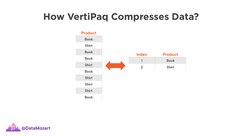
As you may see, VertiPaq will create a dictionary of the distinct values from the column, assign a bitmap index to each of these values, and then store this index value instead of the “real” value – simply said, it will store number 1 as a pointer to “Book” value, number 2 for “Shirt”, and so on. It’s like creating a virtual dimension table in the background!
Now, imagine that instead of two distinct values in the column, we have something like this:
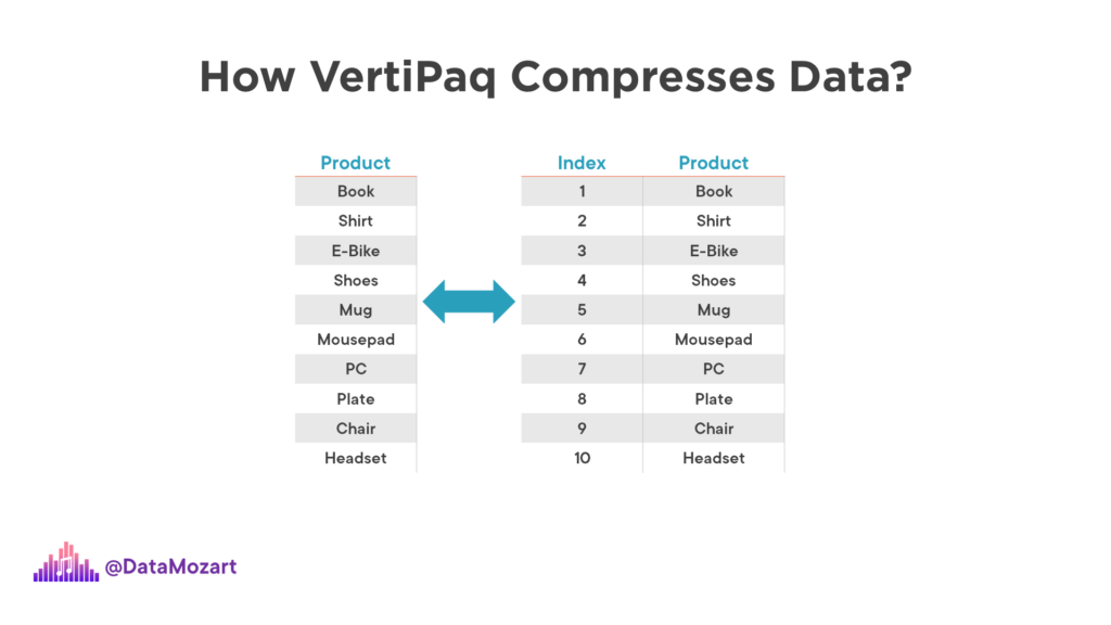
Our “dimension” will now have 10 rows, so you may assume that the size of this dictionary table will be significantly larger than in the previous case with only two distinct values.
Now, you’re probably asking yourselves: ok, that’s fine, but what does all this story has in common with cardinality?
Cardinality represents the number of unique values in the column.
In our first example, we had a cardinality of 2, while in the second case, cardinality equals 10.
And cardinality is the top factor that affects the size of the column. Don’t forget, column size is not affected only by the size of the data in it. You should always take into account dictionary size, same as hierarchy size. For columns that have high cardinality (huge number of distinct values), and are not of integer data type, the dictionary size is significantly larger than the data size itself.
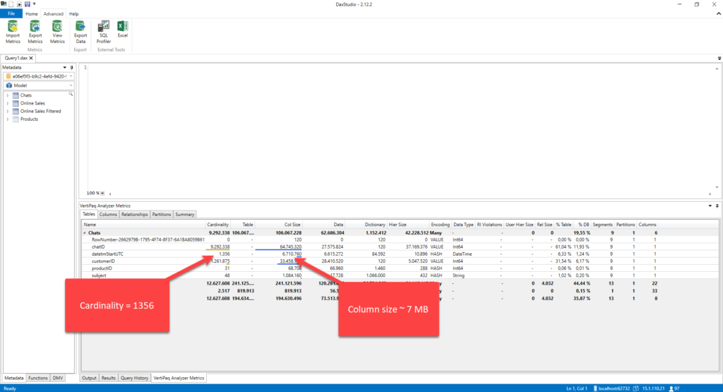
Let me show you one example. I’ll use DAX Studio to analyze different metrics behind my data model size. Once I open the Advanced tab in DAX Studio and select View Metrics, a whole range of different figures will be available, to understand how big are specific parts of my data model:
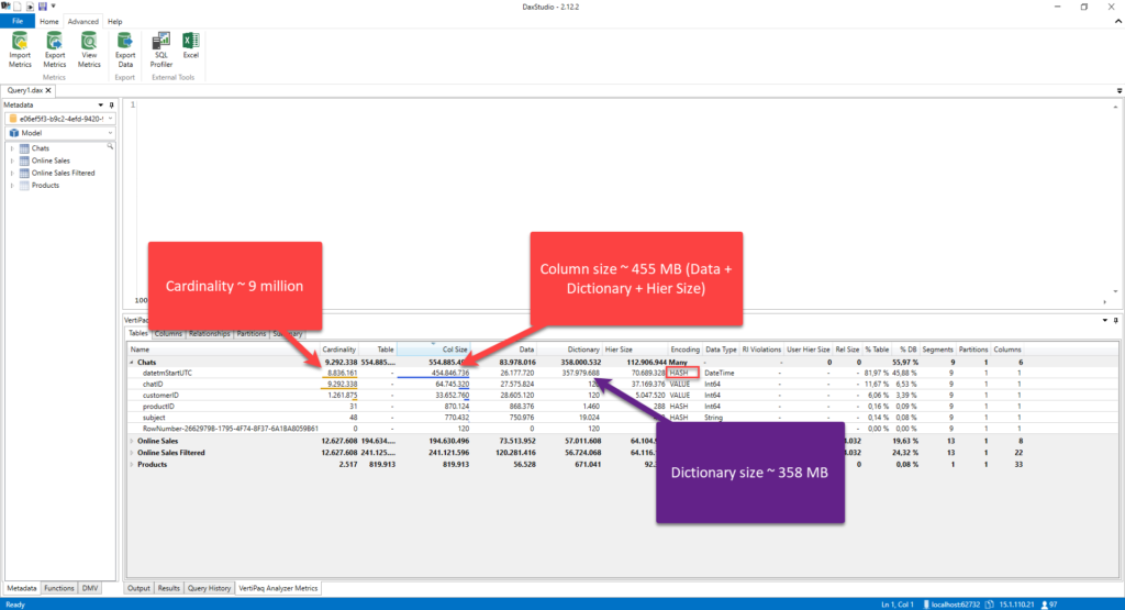
Let’s quickly reiterate the key insights from the illustration above. Within the Chats table, the datetmStartUTC column, which is of Date/Time data type and goes to the second level of precision, has almost 9 million distinct values! Its size is ca. 455 MBs – this figure includes not just data size only, which is 26 MBs, but also dictionary size and hierarchy size. You can see that VertiPaq applied the Hash algorithm to compress the data from this column, but the biggest portion of the memory footprint goes on the dictionary size (almost 358 MBs).
This is, obviously, far from the optimal condition for our data model. However, I have good news for you…
There are multiple techniques to improve the cardinality levels!
In one of the previous articles, I’ve explained how you can reduce the cardinality by applying some more advanced approaches, such as using division and modulo operations to split one numeric column with high cardinality into two columns with lower cardinality and saving a few bits per row. I’ve also shown you how to split the Date/Time column into two separate columns – one containing the date portion only, while the other keeps time data.
However, these techniques require additional effort on the report side, as all the measures need to be rewritten to reflect data model structural changes and return correct results. Therefore, those advanced approaches are not something you’ll need to apply in your regular data model optimization – they are more of an “edge” use-case, when there is no other way to reduce the size of the data model – simply said, when you’re dealing with extremely large datasets!
But, that doesn’t mean that you should not strive to improve the cardinality levels even for the smaller and simpler data models. On the opposite, that should be a regular part of your Power BI development process. In this article, I’ll show you two simple approaches that can significantly reduce the cardinality of the column, thus reducing the overall data model size.
Improve cardinality levels by changing a data type
Let’s be honest – how often do your users need to analyze the data on the second level? Like, how many sales do we have at 09:35:36, or 11:22:48? Makes no sense, I would say. In 98% of cases, the business request is to have data available on a daily level. Maybe in some circumstances, users need to understand which part of the day is the most “productive”: morning, afternoon, or evening…but still, let’s focus on the majority of cases where the data should be grained on a daily level.
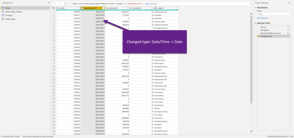
I’ve changed the data type of the column, from Date/Time to Date, as the time portion is irrelevant for reporting purposes. Let’s refresh our metrics in DAX Studio:
Oh, wow! Instead of a cardinality of ~ 9 million, we now have only 1356 (that’s the number of distinct days in the column). But, what’s more important, the size of the column dropped from 455 MB to 7 MB! That’s huuuuge! Look at the dictionary size: instead of having to build a dictionary for 9 million values, VertiPaq now handled just 1356 distinct values, and dictionary size dropped from 358 MBs to 85 KBs!
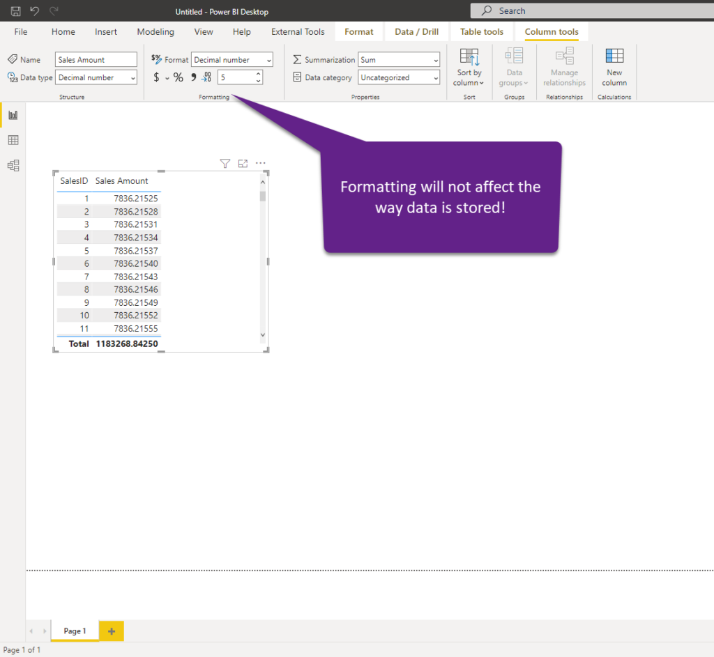
The other trick you can apply is when you’re dealing with decimal values. It’s not a rare situation that you import the data into Power BI “as-it-is” – and, not once, I see people importing the decimal numbers that go to a 5 digit precision after the decimal point! I mean, is it really necessary to know that your total sales amount is 27.586.398,56891, or is it ok to display 27.586.398,57?
Just to be clear, formatting values to display 2 decimal places in the Power BI won’t affect the data model size – it’s just a formatting option for your visuals – in the background, data is being stored with 5 digits after the decimal place.
Now, let’s check the metrics of this table in DAX Studio. This is a trivial data model size, with only 151 distinct values in it, but you can only imagine the difference on multi-million rows table:

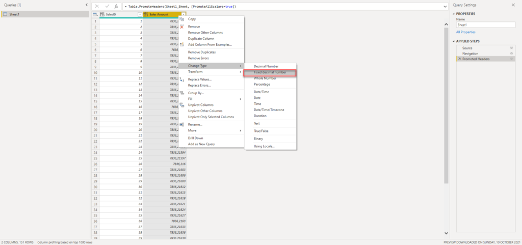
I’ll now go to Power Query Editor and change the type of this column to Fixed Decimal number:
We’ve now rounded values to 2 decimal places after the decimal point, so let’s switch back to DAX Studio and check the numbers again:
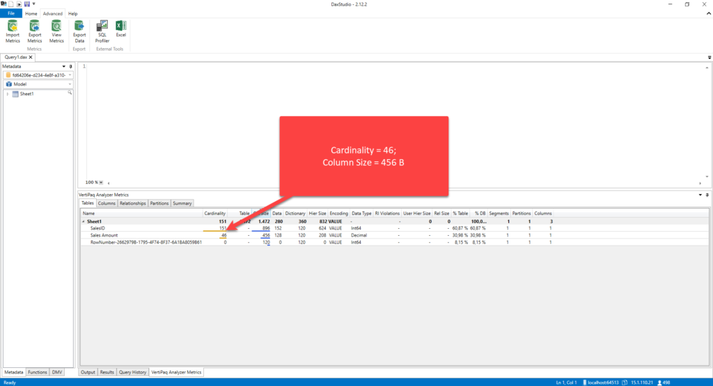
The difference is obvious, even on this extremely small dataset!
UPDATE 2022-11-13: Thanks to Wyn Hopkins, who rightly pointed out that it’s important to keep in mind that Decimal data type goes into 15 decimal places of precision, while Fixed Decimal type stores 4 decimal places, as documented here.
And, if you are now wondering: ok, it’s fine if I round the single transaction value, but how will that affect my calculations? Well, let’s examine one pretty common scenario of calculating the percentage of total for each row in the table:
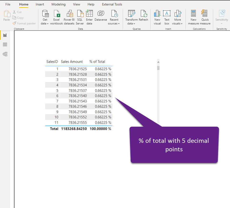
Let’s now check how this calculation works once we reduce the cardinality of the column and round values to two decimal places:
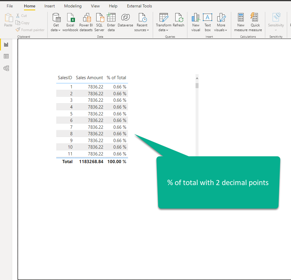
Now, the fair question would be: will business decision-makers care if the share of the individual row is 0.66% or 0.66225%…If these values after the second decimal place are critical for business, then – hell, yes, who cares about the cardinality:)…But, I’d say that in 99.99% of scenarios, no one cares about 0.66 vs 0.66225. In any case, even if someone insists on such precision, try to explain to them all the downsides that higher cardinality brings (memory consumption, slower calculations, and so on), especially on the large fact tables.
Improve cardinality levels using summarization and grouping
The other technique I wanted to show you is how to leverage concepts of summarization and grouping to improve the cardinality levels and make your data model more performant.
When you are creating reports, chances are that the users need to understand different metrics on a higher level of granularity than the individual transaction – for example, how many products were sold on a specific date, how many customers signed up on a specific date, and so on. This means that most of your analytical queries don’t need to target a single transaction, as the summarized data would be completely fine.
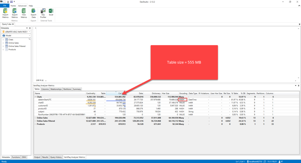
Let’s examine the difference in the memory footprint if we summarize the data for our Chats table. The original table, as you may recall from the previous part of the article, takes 555 MBs:
Now, if I summarize the data in advance, and group it per date and/or product, by writing the following T-SQL:
SELECT CONVERT(DATE,datetmStartUTC) AS datetm
,productID
,COUNT(chatID) AS totalChats
FROM Chats
GROUP BY CONVERT(DATE,datetmStartUTC)
,productID
If the most frequent business requests are to analyze the number of chats per date and/or product, this query will successfully satisfy these requests.
Let’s check the size of this summarized table, compared to the original one:
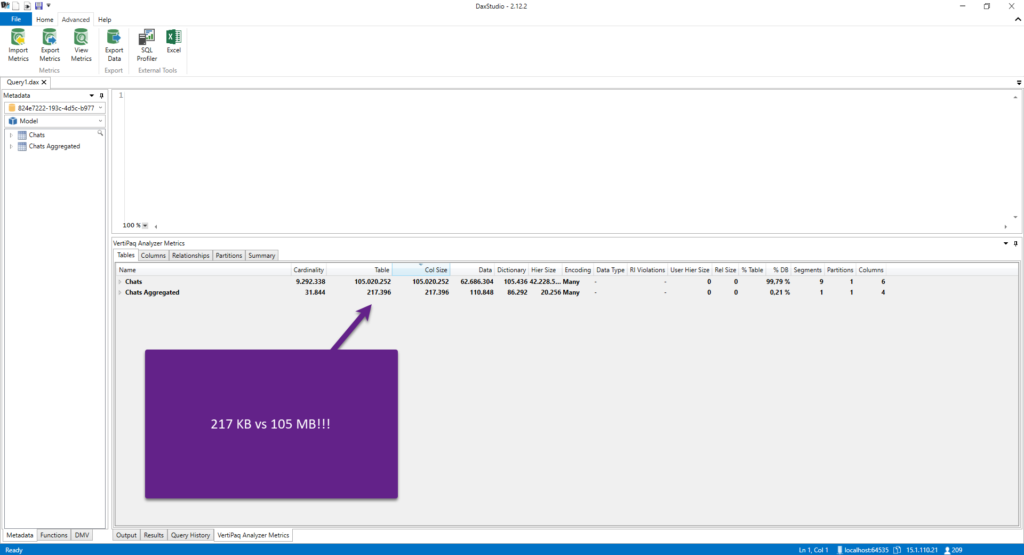
While the original table, even with an improved cardinality level for the datetmStartUTC column, takes 105 MBs, the aggregated table takes only 217 KB! And this table can answer most of the business analysis questions. Even if you need to include additional attributes, for example, customer data, this will still be a more optimal method to retrieve the data.
There is more to this!
Even if you’re not able to create summarized data on the data source side, you can still get a significant performance boost by leveraging the aggregation feature in Power BI. This is one of the most powerful features in Power BI and deserves a separate article, or even a series of articles, like this from Phil Seamark, which I always refer to when I need a deeper understanding of the aggregations and the way it works in Tabular model.
Conclusion
Building an optimal data model is not an easy task! There are many potential caveats and it’s sometimes hard to avoid all the traps along the road to a “perfect” model. However, understanding the importance of reducing the overall data model size is one of the key requirements when tuning your Power BI solutions.
With that in mind, to be able to achieve optimal data model size, you need to absorb the concept of cardinality, as the main factor that determines the column size. By understanding cardinality in a proper way, and the way VertiPaq stores and compresses the data, you should be able to apply some of the techniques we’ve just covered, to improve the cardinality levels of the column, and consequentially, boost the overall performance of your reports!
Thanks for reading!
Last Updated on November 15, 2025 by Nikola


Fernando Calero
Value encoding type can also apply to columns with date data type, correct?
Nikola
Hey Fernando,
I’m pretty sure it can, because dates are internally stored as integers.
Cheers,
Nikola