
A few weeks ago, I was working with a client who needed performance tuning of their Power BI solution. The challenge was to enable the analysis of over 200 million records in the fact table, while ensuring that the lowest level of detail is also available in the report.
Great, that sounds like a perfect use case for Power BI aggregations! I was thinking of aggregating the data per key attributes and then using an Import mode for these aggregated tables – easy win! However, the client insisted that they need to keep the possibility to dynamically choose per which attributes, data will be grouped in the report. Simply said, if I pre-aggregate the data, let’s say, on the product AND store, and they want to include a customer in the scope of the analysis, aggregations would not work in that case, as the grain would be different.
Ok, then let’s use Hybrid tables!
“Look, Nikola, we’ve already heard about the hybrid tables and we think they are super cool…But, there is a “small” issue…We don’t have Premium” 🤔
Not having Premium, also excluded the potential usage of the XMLA endpoint to split the table into two partitions – one that would store the data in Import mode, and the other that will use DirectQuery. The same as in the Hybrid table scenario, but here YOU are in charge of defining partitions.
Oh, that IS a real challenge!
So, no user-defined aggregations, no hybrid tables, no XMLA endpoint…Let’s see what can be done.
What if we “mimic” the behavior of the hybrid table, but without configuring a real one?!
WHAT?! How’s that possible?
Credit: As usual, Phil Seamark came up with a brilliant idea, which you can find on his blog. I leveraged his idea in this specific scenario to make this thing work.
Setting the stage
For the sake of this demo, I’ll use a sample Contoso database that contains ~100 million rows. Courtesy of SQLBI guys (Marco and Alberto), you can generate one for your practice for free!
I’ll keep things simple and I just want to count how many orders were placed for this imaginary Contoso company.
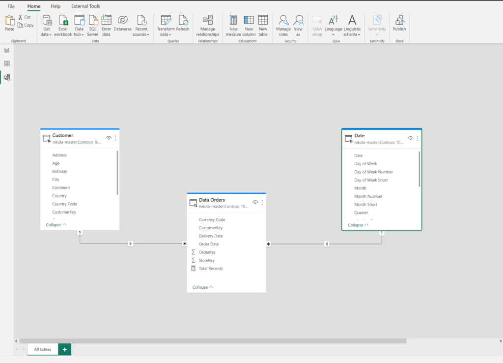
Let me stop for a second and explain the data model (obviously, this is a simplified version of the real data model). There is a fact table Orders and two dimension tables: Customer and Date. All tables are in DirectQuery storage mode, because, as already mentioned, the client needs data on a level of the individual order, and importing 200M+ fact table with a Pro license…Well, it’s simply not feasible.
And, this is how the data in the report looks:
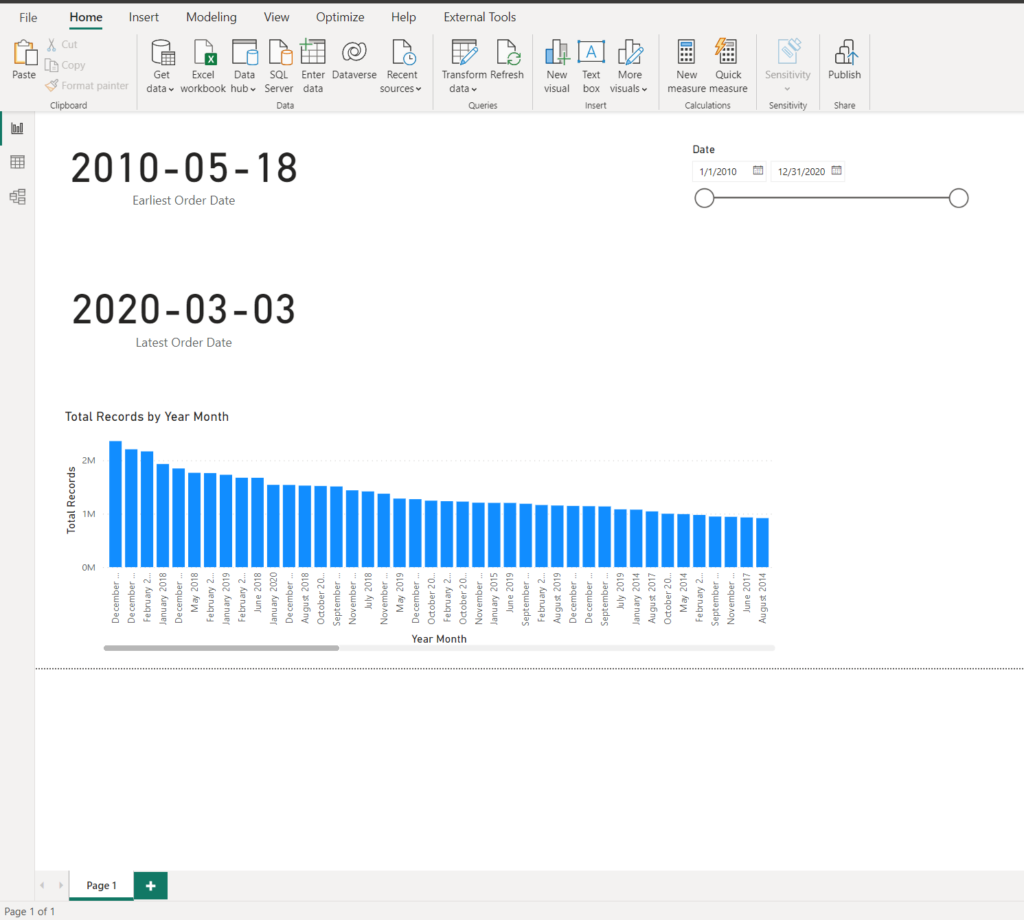
The first order was placed in May 2010, and the last one was on March 3rd 2020. The client explained that most of the analytic queries will usually target the previous three months. Total records is just a simple count of rows from the fact table.
Let’s get to work! Remember when I told you that the idea is to mimic the behavior of the hybrid table. So, obviously, we can’t partition the Orders table, but we can create two tables out of this one – each of them will “act” as a partition!
Now, I hope you are familiar with the terms “hot” and “cold” data – for those of you who are not – “hot” data is the most recent one, where the word “recent” has typical “it depends” meaning. It can be data from the last X minutes, hours, days, months, years, etc. depending on your specific use case. In my case, the hot data refers to all the records from 2020.
Finding the “tipping point” – the point in time to separate “hot” and “cold” data is of key importance here. If you opt to use a shorter period for “hot” data, you will benefit from having a smaller data model size (fewer data imported in Power BI), but you will have to live with more frequent Direct Query queries.
/*Hot data*/
SELECT  [OrderKey]
      ,[CustomerKey]
      ,[StoreKey]
      ,[Order Date]
      ,[Delivery Date]
      ,[Currency Code]
  FROM [Contoso 100M].[Data].[Orders]
  WHERE [Order Date] >= '20200101'
By following the same logic, I’ve created another table to include all the remaining records from the original table, and these records will be stored in the “cold” table:
/*Cold data*/
SELECT  [OrderKey]
      ,[CustomerKey]
      ,[StoreKey]
      ,[Order Date]
      ,[Delivery Date]
      ,[Currency Code]
  FROM [Contoso 100M].[Data].[Orders]
  WHERE [Order Date] < '20200101'
Now, my data model looks slightly different:
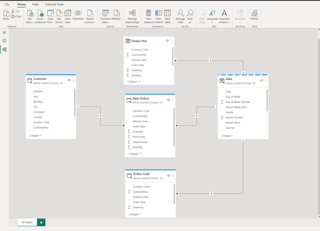
Orders Hot table contains ~3 million rows and is in Import mode, to guarantee the best possible performance. Orders Cold uses, same as the original table, DirectQuery storage mode, as we can’t load such a big table in Power BI without a Premium license. I’ve also set the Date dimension to Dual storage mode, so we avoid all the downsides and challenges of limited relationships.
Since our data model is now essentially structurally different (we have two tables instead of one), I need to rewrite the measure for calculating the total number of orders:
Total Records Hot & Cold = [Total Records Hot] + [Total Records Cold]
Let’s turn on the Performance analyzer in the Power BI Desktop and see what is happening behind the scenes:
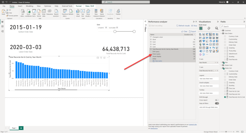
I’ve changed the slicer value to include the data starting from January 19th 2015. Obviously, as we are still retrieving the data from the DirectQuery “cold” table, there is a DirectQuery involved for populating this visual. Please, don’t pay attention to the numbers in this example, as in reality the calculations were more complex and the total time looked much worse:)
Ok, that was somehow expected. But, what happens if I now set my slicer to retrieve the data only from 2020. Remember, we have this data stored in the “hot” table using Import mode, so one would expect to see no DirectQuery here. Let’s check this scenario:
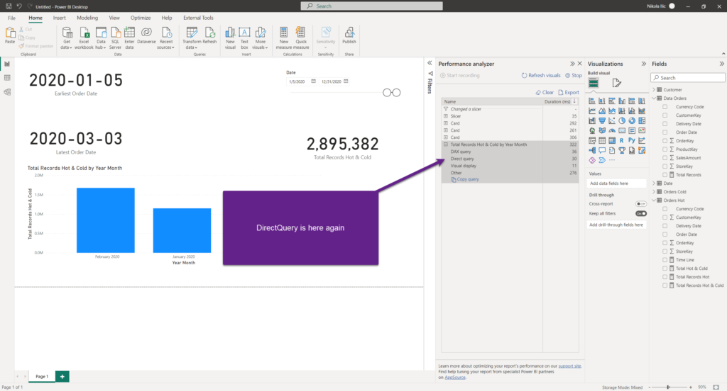
Unfortunately, we have DirectQuery again.
To confirm that, let’s copy the query and jump into the DAX Studio:
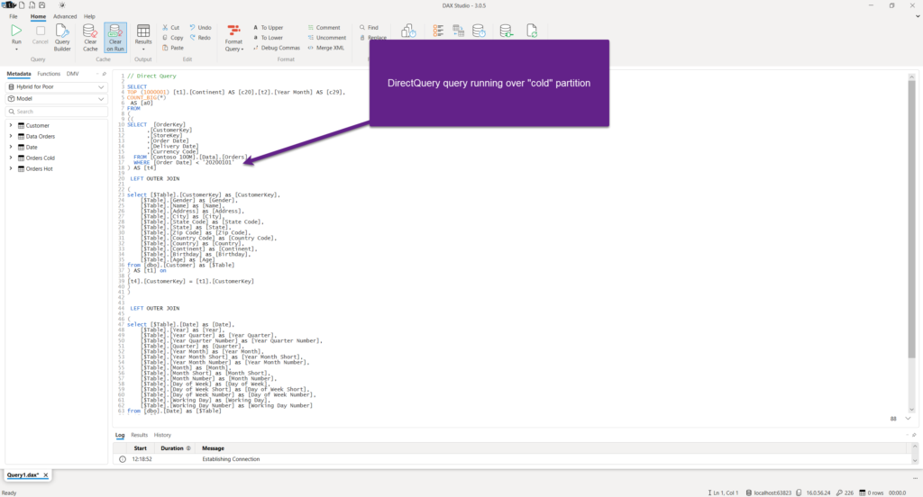
Why on Earth, Power BI needed to apply DirectQuery, when we have our nice little Import table for this portion of the data? Well, the Power BI engine is smart. In fact, it is very smart! However, there are certain situations when it can’t resolve everything on its own. In this scenario, the engine went down and pulled the data even from the “cold” DirectQuery table, and then applied date filters!
That means, we need to “instruct” Power BI to evaluate date filters BEFORE the data retrieval! And, again, thanks to Phil Seamark for the improved version of the measure:)
The first step is to set the “tipping point” in time in DAX. We can do this using exactly the same logic as in SQL, when we were splitting our giant fact table into “hot” and “cold”:
Time Line =
           VAR vMaxDate = CALCULATE(
                                 MAX('Orders Hot'[Order Date]),
                                 ALL()
                                  )
RETURN
    EOMONTH(DATE(YEAR(vMaxDate),MONTH(vMaxDate)-3,1),0)
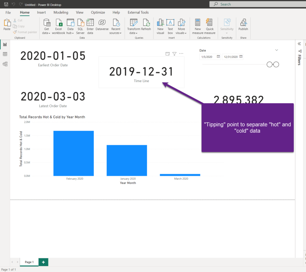
This measure will return the cut-off date between the “hot” and “cold” data. And, then we will use this result in the improved version of our base measure:
Total Hot & Cold =
               VAR vOrdersHot = [Total Records Hot]
               VAR vOrdersCold = IF(
                                     MIN('Date'[Date]) <= [Time Line] ,
                                     [Total Records Cold]
                                   )
RETURN
vOrdersHot + vOrdersCold
Here, we are in every scenario returning the total number of orders from the “hot” table, as it will always hit the high performant table in Import mode. Then, we are adding some logic to “cold” data – checking whether the starting date in the date slicer is before our “tipping point” – if yes, then we will need to wait for the DirectQuery.
But, if not, well…
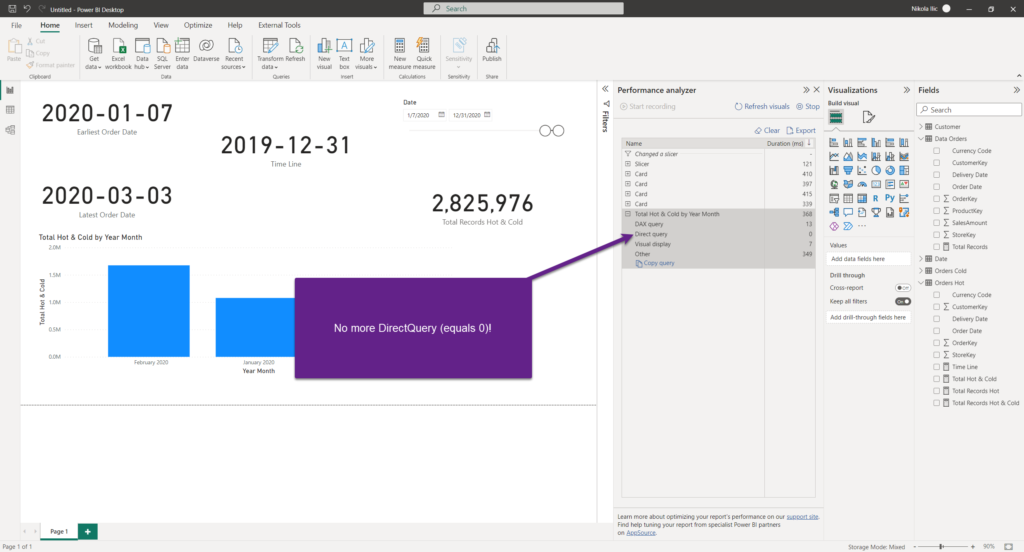
Let’s again copy the query and check it in DAX Studio:
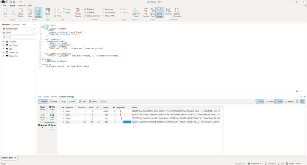
No DirectQuery query at all! Only DAX!
Do you know what’s even better? Remember that one of the client’s requests was to be able to dynamically choose the attributes within the visuals? So, once I include the continent in the scope, let’s see what is going to happen:
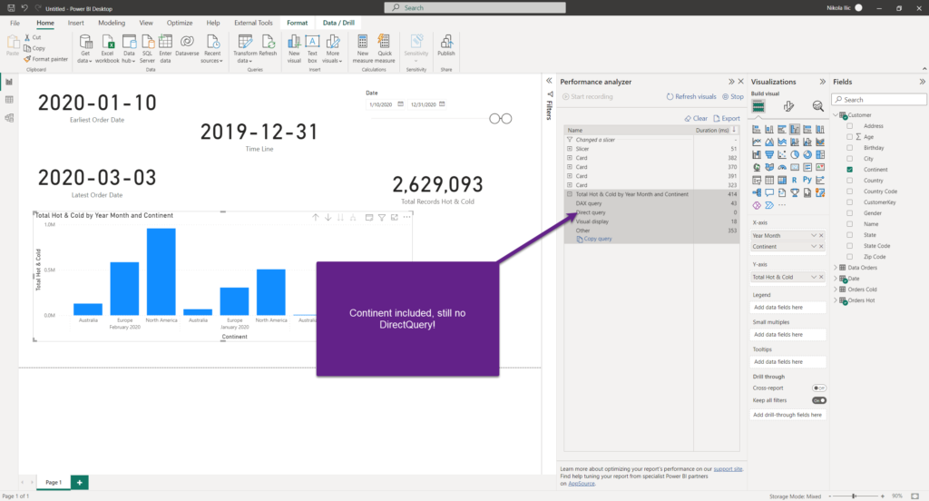
Worked like a charm! As long as the data is coming ONLY from the import table, there will be no DirectQuery queries anymore.
Conclusion
As you witnessed, we made it! The original request was to enable data analysis over 200M+ records in the most efficient way, additionally supporting the dynamic selection of attributes for analysis. No Premium – no problem! We managed to keep the original data granularity, while increasing the report performance for 99% of use cases!
Extraordinary tasks require extraordinary solutions – and, if you ask me, thanks to Phil Seamark’s brilliant idea – we have a solution to accommodate extremely large data even into Pro limits, without sacrificing the performance.
Thanks for reading!
Last Updated on February 1, 2023 by Nikola