
This article is the part of the series related to mastering DP-500 certification exam: Designing and Implementing Enterprise-Scale Analytics Solutions Using Microsoft Azure and Microsoft Power BI
Table of contents
“DAX is simple, but not easy!” – famously said Alberto Ferrari, when asked which best describes Data Analysis Expression language. And, that’s probably the most precise definition of the DAX. It may look very easy at first glance, but understanding nuances and how DAX really works, requires a lot of time and “try and fail” cases.
Obviously, this article is not a deep-dive into DAX internals and will not go into these nuances, but it will (hopefully) help you to get a better understanding of the few very important concepts that will make your DAX journey more pleasant and assist you in preparing the DP-500 exam.
Variables in DAX
As a DAX newbie, it’s easy to fall into the trap of thinking that you don’t need variables. Simply said, why would you care about the variables when your DAX formulas consist of one or two lines of code?!
However, as time goes by, and you start writing more complex calculations, you’ll start to appreciate the concept of variables. And, when I say more complex calculations, I mean using nested functions, and possible reusing of the expression logic. Moreover, in many cases variables may significantly improve the performance of your calculation, as the expression will be evaluated by the engine only once, instead of multiple times!
Finally, using variables enables you to easier debug the code and verify results for the certain part(s) of your formula.
Here is the simple example of using variables in your DAX code:

As you may notice, defining variables requires usage of the var keyword before the expression to be evaluated and assigned to a specific variable.
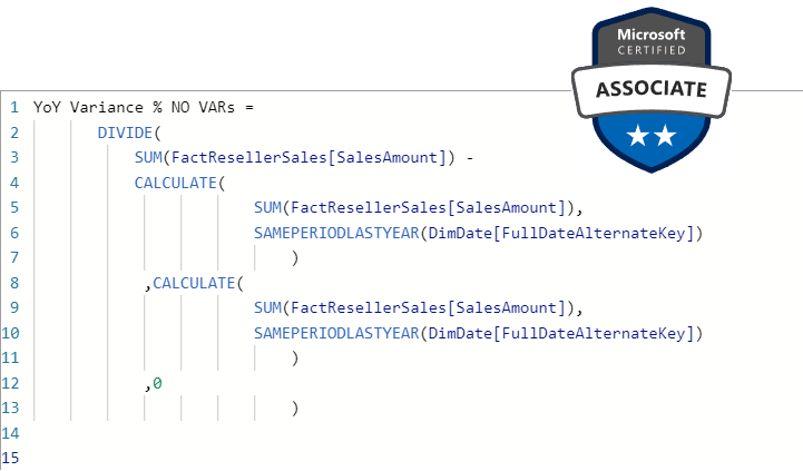
Of course, the example above is fairly simple, but let’s imagine that we want to display YoY Variance as a percentage. We can write a measure like this:

The first thing to spot here is that we are repeating exactly the same expression for calculating the sales amount for the previous year. We could’ve written the same measure this way:
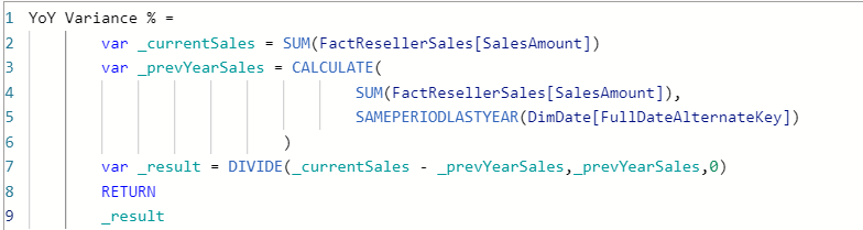
I guess we agree that the second version is way more readable and easier to read and understand. As I said, this was a fairly basic formula, you can just imagine the impact of using variables in more complex scenarios, with nested functions.
Variables can be used both in measures and calculated columns.
Handling Blanks
While creating reports, I’m sure that you are facing situations when you get (blank) as a result and you don’t want to display it like this to your end users.
I’ve already written an article that shows three possible ways to handle BLANKs in your Power BI reports.
You can choose between using IF statement, COALESCE() function, or applying trick with adding 0 to your numeric calculation.
However, in another article, I’ve also explained why should you think twice before replacing blanks with some other values. In certain scenarios, this can be a real performance killer.
Virtual Relationships in DAX
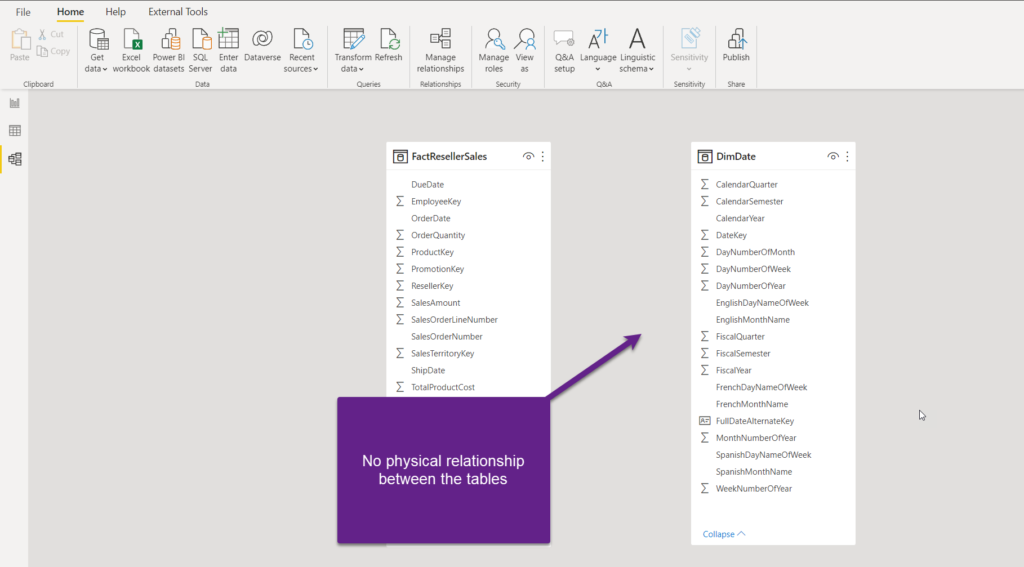
Before I explain what are virtual relationships and how to create them, I’d like to emphasize that having a physical relationship between the tables in the data model is always a recommended practice! However, in some circumstances, it may happen that you don’t have a physical relationship between the tables, and you simply need to simulate the non-existing physical relationship.
The most convenient way to create a virtual relationship is using TREATAS() function in DAX. As explained in this article from SQL BI, this is how the pseudocode for creating a virtual relationship with TREATAS would look like:
[Filtered Measure] :=
CALCULATE (
    <target_measure>,
    TREATAS (
        SUMMARIZE (
            <lookup_table>
            <lookup_granularity_column_1>
            <lookup_granularity_column_2>
        ),
        <target_granularity_column_1>,
        <target_granularity_column_2>
    )
)
Let’s see how this looks on a real-life example! I’ll show you how virtual relationships can be leveraged in a role-playing dimension scenario. Unlike in one of the previous articles, where I explained how to handle role-playing dimensions using USERELATIONSHIP() function to change the active relationship between the tables, I’ll now show you how to create two virtual relationships between the tables that are not connected with the physical relationship in the model:
Let’s say that I want to analyze how many orders were placed on a specific date (OrderDate) vs how many orders were shipped on a certain date (ShipDate). The first measure will establish the virtual relationship between the FactResellerSales and DimDate table on the OrderDate column:
Total Quantity Order Date =
                CALCULATE(
                            SUM(FactResellerSales[OrderQuantity]),
                            TREATAS(
                                VALUES(DimDate[FullDateAlternateKey]),
                                FactResellerSales[OrderDate]
                            )
                )
Essentially, as a lookup table for our virtual relationship, by using VALUES() function, we are taking all the distinct (non-blank) values from the DimDate table. On the other side of this virtual relationship is our OrderDate column. Let’s create a similar measure, but this time establishing a virtual relationship on the ShipDate column:
Total Quantity Ship Date =
                CALCULATE(
                            SUM(FactResellerSales[OrderQuantity]),
                            TREATAS(
                                VALUES(DimDate[FullDateAlternateKey]),
                                FactResellerSales[ShipDate]
                            )
                )
This is how our table visual looks after we put both measures on it:

So, even though our tables are not related with a physical relationship, we were able to create relationships “on the fly” and display correct numbers in the Power BI report.
DAX Iterators
Unlike aggregators, that aggregate all the values from the specific column and return a single value, iterators apply expression for each row of the table they are operating on!
Therefore, the first difference between the two is that iterators need (at least) two parameters to work – the first is always a table that they need to iterate on (both physical or virtual table), and the second is the expression that needs to be applied for every row of that table.
The most common iterator functions are actually the “relatives” of the aggregator functions:
| Aggregator Function | Iterator Function |
| SUM | SUMX |
| AVERAGE | AVERAGEX |
| MIN | MINX |
| MAX | MAXX |
As you see, iterator functions has letter X in the end and that’s the easiest way to recongize them within the DAX formula. However, it’s an interesting fact that aggregator functions are internally translated by engine to iterator function too! So, when you write something like:
Sales Amount = SUM('Online Sales'[SalesAmount])
It’s internally translated to:
Sales Amount = SUMX('Online Sales',
                     'Online Sales'[SalesAmount]
                 )
Please keep in mind that whenever you want to write an expression that includes more than a single column, you MUST use iterators!
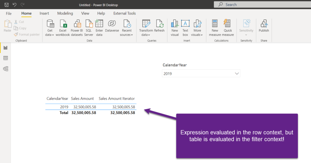
The key thing to understand with iterator functions is the context in which they are operating. As they are iterating row by row, the expression is evaluated in the row context, similar to calculated column DAX formula. However, the table is evaluated in the filter context, which means that if, let’s say, there is an active filter on the ‘Online Sales’ table to show only the data from year 2019, the final result will include sum (assuming that you’re using SUMX iterator function) over the rows from year 2019.
Sales Amount Iterator =
                    SUMX (
                        FactResellerSales,
                        FactResellerSales[OrderQuantity] * FactResellerSales[UnitPrice]
                    )
The final warning regarding the iterator functions: be careful when using complex iterator functions over large amounts of data, as they are being evaluated row-by-row, and may cause performance issues in some cases.
Conclusion
Keep repeating: “DAX is simple, but not easy!”…As you may’ve seen, DAX offers you a quick entry into the world of (im)possible – where you can perform all kinds of calculations, but you need to be aware of the language nuances and understand how the engine really works in the background.
I strongly suggest following SQL BI channel and blog, or even better, reading a “DAX bible“: The Definitive Guide to DAX, 2nd edition.
There are also other fantastic resources on the web for learning DAX, such as Enterprise DNA channel, or Brian Grant’s awesome series of videos, called “Elements of DAX“.
Thanks for reading!
Last Updated on January 20, 2023 by Nikola


