TIQ Part 4 – Being Time intelligent

TIQ stands for Time Intelligence Quotient. As “regular” intelligence is usually being measured as IQ, and Time Intelligence is one of the most important topics in data modeling, I decided to start a blog series which will introduce some basic concepts, pros and cons of specific solutions and potential pitfalls to avoid, everything in order to increase your overall TIQ and make your models more robust, scalable and flexible in terms of time analysis

• TIQ Part 1 – How to destroy your Power BI model with Auto Date/Time
• TIQ Part 2 – Your Majesty: Date Dimension
• TIQ Part 3 – Ultimate Guide to Date dimension creation

Dear reader, we are closing to an end of this series. After a detailed explanation of why you can, but you shouldn’t, use Auto Date/Time feature in Power BI, then underlying the significance of Date dimension within your data model, in the previous article I’ve offered you various solutions for creating a proper Date dimension.

So, it’s time to wrap-up with some examples of the most frequently used time-related calculations and some neat differences between them.

What is Time Intelligence?

In the simplest way, Time Intelligence represents some kind of calculation related to dates. Don’t let to be confused with the word “Time” and expect to see hours/minutes/seconds/milliseconds as the lowest level of granularity when someone talks about “Time intelligence”.

The more appropriate term would be “Date Intelligence”, but since “Time Intelligence” is already generally accepted, let’s stick with this naming convention.

The main characteristic of all Time Intelligence functions in DAX is that one way or the other, they need to operate on a column of Date or Date/Time data type. This means that one of the input parameters for these functions needs to be the Date or Date/Time column.

Also, all of them will shift your selected dates into some new dates (be it in the past or in the future).

Last, but not least, Time intelligence functions support the single day as the lowest level of granularity – this means that you can’t use them in calculations for hours/minutes/seconds, etc.

Check-list for proper usage of Time Intelligence functions

• As stressed in previous articles of this series, you should create a separate Date dimension, following all the necessary rules (contiguous dates, unique values, non-NULL values, etc.)
• Create a relationship between Date dimension and Fact table(s) on a column of data types Date or Date/Time, not on surrogate key integer columns, unless you mark your Date dimension as a Date table (in that case creating relationship on integer surrogate keys is also fine) Thanks to Derek van Leeuwen, MSc for spotting previously imprecise explanation
• Don’t use your Date or Date/Time columns from a fact table(s) in Time intelligence functions (for example, don’t use column Order Date from Fact Online Sales table from our sample Contoso database)
• Always create full year values in your Date dimension. That means, even if you have last order in the fact table in September 2013, your Date dimension should include whole 2013 year, with December 31st as the last value
• As mentioned in the previous chapter, stick to the single day as the lowest level of granularity

Most common Time intelligence functions

There are dozen of Time intelligence functions, but some of them are being used more frequently than the others. For example, almost every Power BI report that operates with numbers needs some kind of comparison in order to identify trends. Or, displaying cumulative values is also one of the top business requests.

These functions look simple at first glance, but at the same time, they are quite powerful. Let’s look at this simple example of calculating running totals for the selected year.

In the Contoso database, I’ve created measure to calculate Sales Amount:

 Sales Amt = SUM('Online Sales'[SalesAmount])

Now, let’s create our measure for calculating running totals:

Sales Amt YTD = CALCULATE('Online Sales'[Sales Amt],
DATESYTD(Dates[Date])
)

When I drag these measures to a report and select months from January to August 2009, you can immediately notice the difference in numbers on month level:

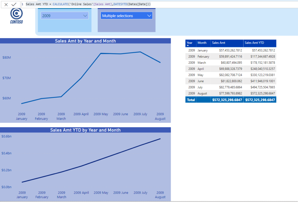
That was quite straightforward, but let me explain what is happening in the background of Sales Amt YTD measure calculation because that is quite important in order to understand the whole logic here.

Going beyond basics

Recall the time-shifting concept I’ve mentioned above – here, we selected dates from January 1st 2009 to August 31st 2009. What is happening for YTD calculation is that the filter context is changed to include dates between January 1st 2009 and the last day of the selected month, no matter which month we selected!

This is gonna be much more clear looking at the following example, where I selected months from March 2009 to August 2009:

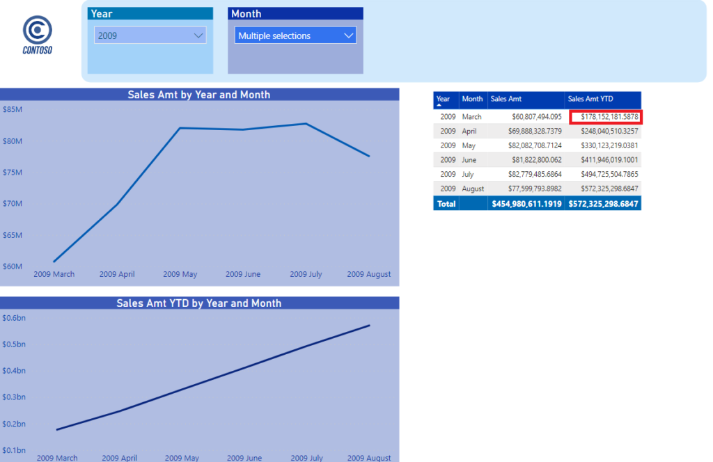
Take a careful look at the value marked in red. No matter we selected March to display our numbers, DATESYTD() function resets our filter and includes values from the beginning of the year. We don’t see them in the table, but they are included in the March totals, as you can easily compare with the first screenshot. Totals for YTD remained unchanged, no matter we changed our selection in the slicer.

One of the things I like most in DAX is the fact that you can achieve same goals in multiple different ways. That also stands for running totals calculations, since instead of DATESYTD(), you can also use TOTALYTD() function. TOTALQTD() and TOTALMTD() works in the same manner, but on different granularity (quarters and months respectively).

Devil is in the details…

You should also pay attention to neat differences between specific functions, because in one scenario they can give you exactly the same results, but then to perform completely different in some other situations.

Therefore, if you want to perform Year-Over-Year comparisons, you can use both SAMEPERIODLASTYEAR() and DATEADD() functions, and following measures…

Sales Amount PY = CALCULATE(SUM('Online Sales'[SalesAmount]),
DATEADD(Dates[Date],-1,YEAR)
)

Sales Amount PY Alt = CALCULATE('Online Sales'[Sales Amt], 
SAMEPERIODLASTYEAR(Dates[Date])
)

…will return the same results:

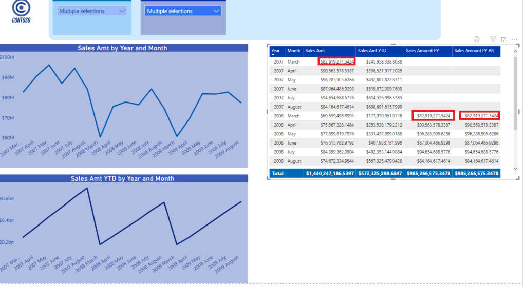
The only difference is that DATEADD() gives you more flexibility since you can shift intervals according to your needs and on different levels of Date hierarchy (quarters, months, days), while SAMEPERIODLASTYEAR() is bounded to previous year only. PARALLELPERIOD() is also very similar, but still different enough, in the way that we are setting static interval for date shifting:

Sales Amount PP = CALCULATE('Online Sales'[Sales Amt],
PARALLELPERIOD(Dates[Date],-12,MONTH)
)

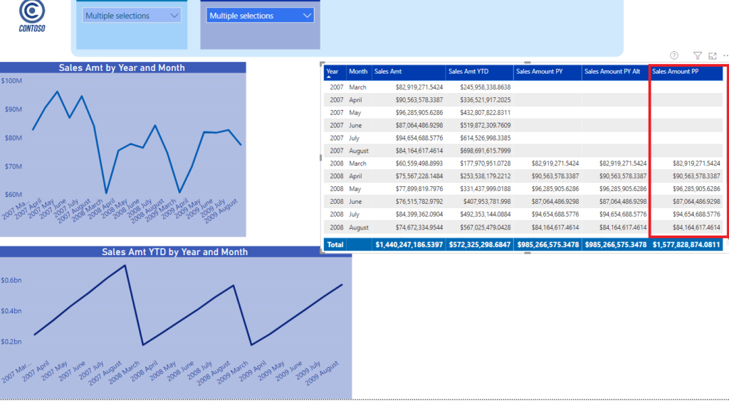
But, as we change last created measure to…

Sales Amount PP = CALCULATE('Online Sales'[Sales Amt],
PARALLELPERIOD(Dates[Date],-1,YEAR)
)

…you would expect that -1 YEAR relates to -12 MONTHS…

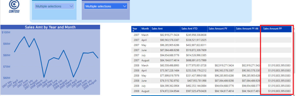
However, that is not the case, as PARALLELPERIOD will return total Sales Amount for the whole previous year (slicer selection has been disregarded):

I don’t want to say: use DATEADD() and don’t use PARALLELPERIOD(). Or, avoid SAMEPERIODLASTYEAR() and use instead DATEADD(). All of these functions have their place in your calculations – key takeover here is: be careful when you’re selecting Time intelligence functions for performing specific time calculations! As you’ve already seen, in some cases they will all return the same results, but in reality, they behave completely differently.

Conclusion

Time Intelligence is one of the most important concepts in Power BI (and Business Intelligence in general). Therefore, it’s almost impossible to cover all stuff in few blog posts, as I boldly tried. However, I sincerely hope that some basic concepts and ideas are more clear now.

In the end, I bet that your TIQ (Time Intelligence Quotient) is higher than it was when you started this (hopefully) interesting TIQ journey.

Thanks for reading!

Last Updated on July 14, 2020 by Nikola