Mastering DP-600 Exam: DAX For The Win Part 2 – Window Functions and Information Functions

This article is part of the series related to mastering the DP-600 certification exam: Implementing Analytics Solutions Using Microsoft Fabric

Disclaimer: The official skill measured in the DP-600 exam is called: Write calculations that use DAX variables and functions, such as iterators, table filtering, windowing, and information functions. However, I’ve decided to split this into two separate articles – in this one, I’ll cover Window and Information functions, whereas, in the previous one, I’ve covered variables and iterators

Window functions

If you’re coming from the SQL world, you might have already heard about window functions. However, window functions are relatively new enhancement in the DAX language. Similar to SQL, they aim to provide the possibility to calculate specific expressions over a sorted and partitioned set of rows.

I’ve already written an article explaining how you can leverage window functions to calculate Customer lifetime value for your business.

If you want to learn more about these functions and how they work behind the scenes, I strongly recommend reading this article from Jeffrey Wang – this is the best starting point for diving deeper into DAX window functions.

Three main DAX window functions are:

INDEX
OFFSET
WINDOW

By leveraging these functions, you can easily calculate something like:

Sorting customers by the total amount spent, and comparing the current customer with the previous customer
Compare the sales from the current year and the previous year
Calculating moving averages or running totals in a window of N quarters, months, days…

When you use window functions, it’s important to understand their arguments – ORDERBY and PARTITIONBY. PARTITIONBY determines the “window” itself, or simply said, the subset of rows that you want to apply the calculation on, whereas ORDERBY defines the sorting order of the results within the “window”.

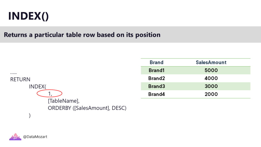
INDEX Function

Let’s first introduce the INDEX function. This function simply returns a particular row of the table based on its position. For example, if you want to return the brand with the highest sales, you can use the INDEX function and specify number 1 for the best-performing brand. In case you want to return the 2^nd highest-performing brand, then you simply modify the numeric value in the first argument of the INDEX function.

In this example, we haven’t used PARTITIONBY clause, which means that we performed our calculation on the entire table. Now, let’s imagine that we need to identify the highest-selling brand within each category. So, not the overall highest-selling brand, we already calculated that, but the top performer in each category, such as Audio, Computers, and so on…

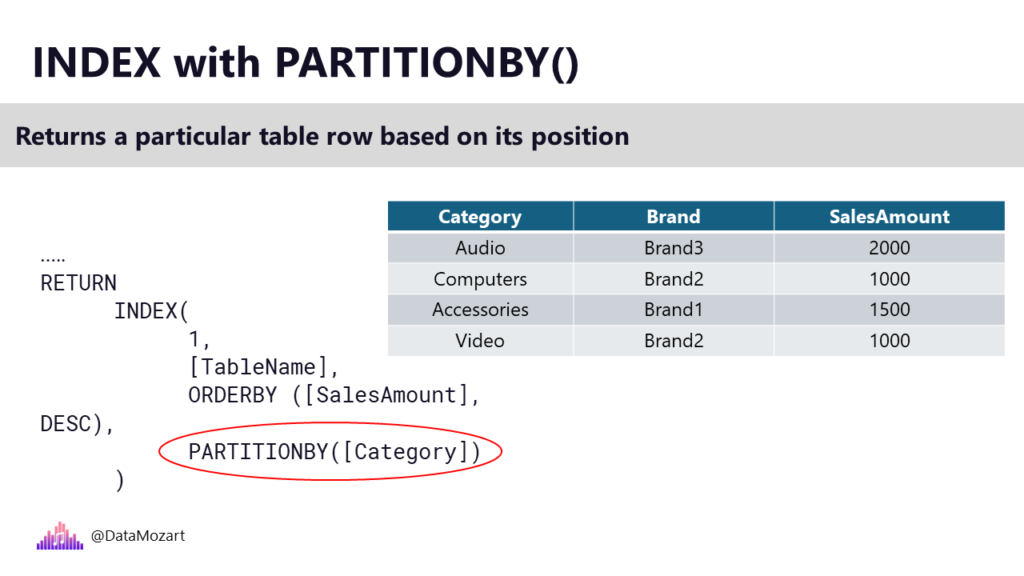
PARTITIONBY will create smaller sub-tables within the main table, and then we perform our calculation in the scope of each of these smaller sub-tables.

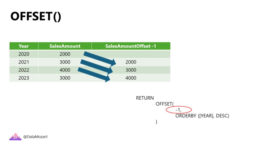
OFFSET Function

OFFSET function returns the row relative to the current row. The first argument instructs how many rows we need to move forward or backward from the current row.

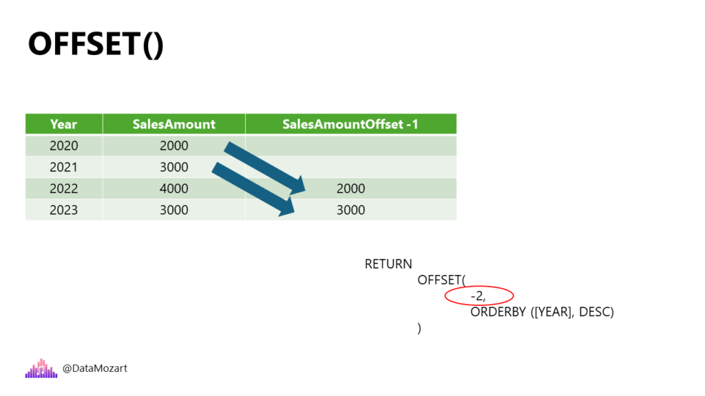
Let me show you a very simple example of the OFFSET function. We have a basic table, which shows the total sales amount for each year. Now, we need to include the value for the previous year. If I pass -1 as a value of the first argument, the calculation will refer to the value from the previous cell. If we change this to -2, it will move backward for two cells, and so on…

OFFSET function with -1 shows the value from the previous cell

OFFSET function with -2 shows the value from two cells backward

WINDOW Function

Finally, the WINDOW function is the most complex one. It enables defining the window based on the current row using either relative or absolute references. Again, let’s explain how this function works in a real-life example.

I’m analyzing two customers from the Adventure Works dataset: Adam Young and Alexandra Jenkins. Here is the summary of their orders and total sales amount:

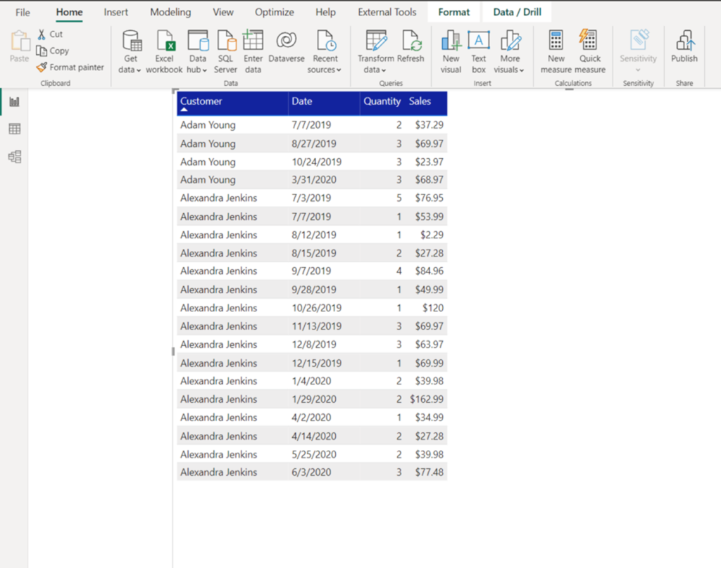
The first concept to understand here is that we want to treat each customer as a separate “entity” – meaning, we want to create a “window” for each customer and analyze figures for that specific set of rows. In our case, we will have two “windows” here:

Window functions in DAX can work in two different ways – either by operating on a relative (REL) value, based on the current row, or by operating on an absolute (ABS) value. In my case, I always want my window to start at the first row of the partition (each customer represents a separate partition), and finish on the last row of the partition.

So, let’s create a measure that will calculate a running total of order quantity and sales for every partition:

Window Sales Amount = CALCULATE([Total Sales],
                             WINDOW(
                                 1,ABS,
                                -1,ABS,
                                SUMMARIZE(
                                     ALLSELECTED(Sales),
                                     Customer[Customer],
                                     'Date'[Date]
                                         ),
                        ORDERBY ('Date'[Date]),
                        KEEP,
                        PARTITIONBY(Customer[Customer])
                                  )
                   )

Let’s stop for a moment and explain this measure definition.

As a CALCULATE filter modifier, we’re going to use the WINDOW function. The first argument (1) determines where the window starts. Because the second argument is ABS (absolute), this means that the window starts at the beginning of the partition. Next, we define where the window ends. Since we are using a negative value (-1) and ABS, this means that the window ends in the last row of the partition. After that, we are defining a table expression from which the output row will be returned. Finally, data will be sorted by date within the window (starting with the earliest date), and partitioning will be performed on a customer (each customer is a separate “window”).

DAX Information Functions

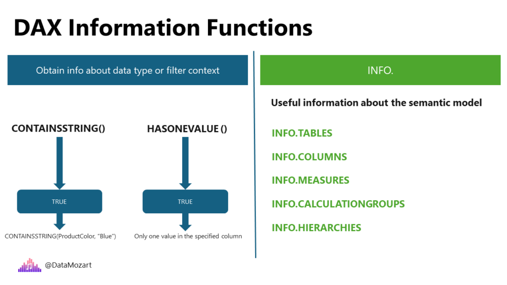
Information functions in DAX can be used in multiple scenarios. The most common scenario is when you need to obtain information about the data type or filter context. For example, CONTAINSSTRING function will return TRUE if one text string contains another text string. Or, HASONEVALUE, which evaluates to TRUE if there’s only one value in the specified column. Additionally, there is a group of information functions that perform logical checks and return TRUE/FALSE as a result of these checks. Some of the most frequently used functions are ISBLANK, ISEMPTY, ISERROR, ISFILTERED, ISINSCOPE, and so on.

Another group of information functions starts with the keyword INFO. By leveraging these functions, you can obtain various useful information about your semantic model and its core elements, such as tables, columns, measures, calculation groups, data sources, hierarchies, and many more.

I found these functions particularly useful in the following two scenarios:

Identifying measures without description – a recommended practice is to have a proper description of each measure in your semantic model, so that users understand its purpose and the logic behind a specific calculation. Hence, you can write the following DAX code, leveraging INFO.MEASURES function

EVALUATE
    INFO.MEASURES()

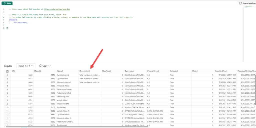
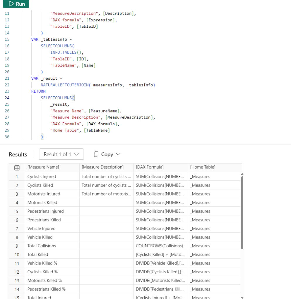
Apparently, a lot of columns returned might not be super useful (such as ID, or TableID), so we can narrow down results to what’s really needed:

EVALUATE
    VAR _measuresInfo = 
        SELECTCOLUMNS(
            INFO.MEASURES(),
            "MeasureName", [Name],
            "MeasureDescription", [Description],
            "DAX formula", [Expression],
            "TableID", [TableID]
        )
    VAR _tablesInfo = 
        SELECTCOLUMNS(
            INFO.TABLES(),
            "TableID", [ID],
            "TableName", [Name]
        )
    VAR _result = 
        NATURALLEFTOUTERJOIN(_measuresInfo, _tablesInfo)
    RETURN
        SELECTCOLUMNS(
            _result,
            "Measure Name", [MeasureName],
            "Measure Description", [MeasureDescription],
            "DAX Formula", [DAX formula],
            "Home Table", [TableName]
        )

Finding all calculated columns in the semantic model – I’m a big fan of doing all the transformation logic “as upstream as possible” (“Roche’s Maxim”), so I really try to stay away from using DAX calculated columns. Discussing the pros and cons of DAX calculated columns is out of the scope of this article. The focus is on quickly identifying these columns in the model

DEFINE
    VAR _tablesInfo = 
        SELECTCOLUMNS(
            FILTER(
                INFO.TABLES(),
                // Exclude hidden tables
                [IsHidden] = FALSE()
            ),
            "TableID",[ID],
            "TableName",[Name]
        )
    VAR _columnsInfo = 
        FILTER(
            INFO.COLUMNS(),
            // Exclude RowNumber columns
            [Type] <> 3
            ) 
    
    VAR _result = 
        SELECTCOLUMNS(
            NATURALINNERJOIN( 
                _columnsInfo,
                _tablesInfo
            ),
            "Table Name",[TableName],
            "Column Name",[ExplicitName],
            "Description",[Description],
            "Source Column",[SourceColumn],
            "Column Type", 
                SWITCH(
                    [Type],
                    1,"Data column", 
                    2, "Calculated column",
                    [Type]
                ),
            "DAX formula", [Expression]
        )
EVALUATE
        FILTER(
    		_result,
			[Column Type] = "Calculated column"
		)

Conclusion

Window functions in DAX open up a whole new world of possibilities for more flexible and powerful data analysis. Not just that, these functions are at the core of Visual Calculations, one of the latest additions to Power BI, which enables self-service business users to perform more intuitive calculations in their Power BI reports. You can learn more about Visual Calculations her e.

Information functions are useful for understanding the data type or the filter context, whereas INFO functions provide details about various semantic model objects, such as tables, columns, measures, calculation groups, and many more.

Thanks for reading!