Looking through the WINDOW – Calculating customer lifetime value with new DAX functions!

In my previous “life” as a SQL professional, I’ve been using T-SQL window functions extensively for various analytic tasks. I’ve described one of the possible use cases in this article, but there are literally dozen of scenarios that can be quickly and intuitively solved by using window functions.

Therefore, when I transitioned to Power BI, I was quite surprised (not to say disappointed) that there is no DAX equivalent to SQL window functions. Ok, we could have solved these challenges of performing different calculations over a certain set of rows, by writing more complex DAX – but, honestly, that was very often a really painful experience.

So, I was beyond excited when Power BI Desktop December 2022 update announced a brand new set of DAX functions – collectively called window functions – that should achieve the same goal as SQL window functions. At this moment, there are three DAX window functions: OFFSET, INDEX, and WINDOW.

If you want to learn more about these functions and how they work behind the scenes, I strongly recommend reading this article from Jeffrey Wang – this is the best starting point for diving deeper into DAX window functions.

If you’re specifically interested in the OFFSET function, I encourage you to read this great article written by my friend Tom Martens, or this one by Štěpán Rešl.

In this article, I’ll not spend too much time explaining the ins and outs of the window functions, as I want to focus on explaining how you can leverage these functions to satisfy a very common business request – calculate the lifetime value of the customer.

Customer lifetime value

Let’s start with understanding what is a customer lifetime value. Well, it’s a broad term and may be interpreted in many possible ways. In our case, we want to provide a deep insight into the behavior of a single customer – for example, how many orders they placed, what is the total amount they spent on our products, how many days passed between their orders, and how this compares to the average of all customers. Finally, we want to know how loyal are our customers – meaning, how many days passed between their first and last order.

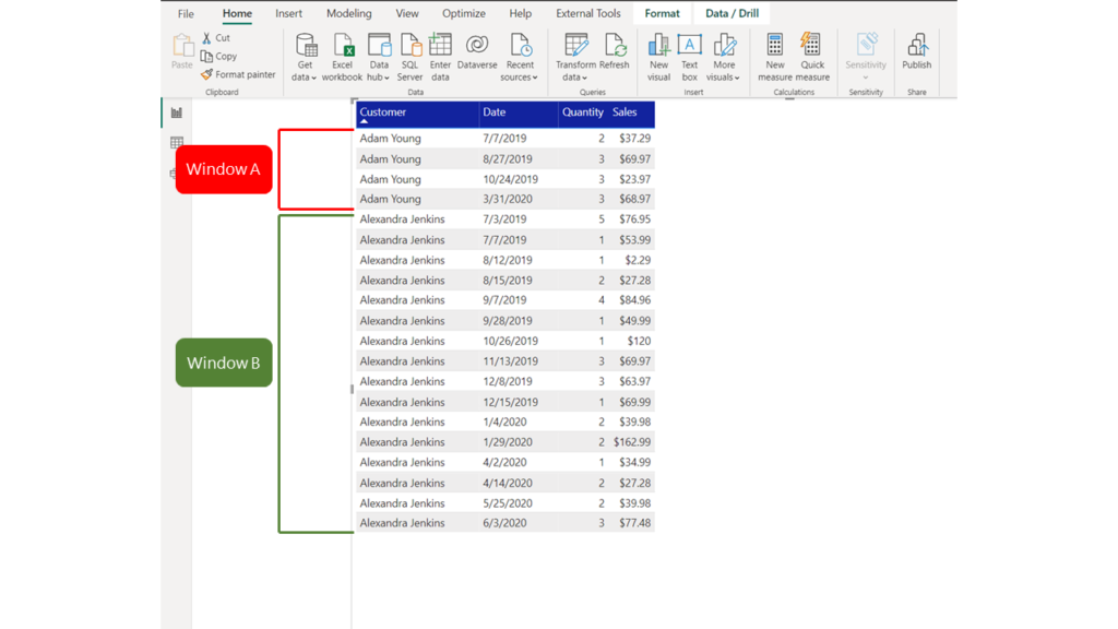
So, let’s begin with a very basic scenario. I’m analyzing two customers from the Adventure Works dataset: Adam Young and Alexandra Jenkins. Here is the summary of their orders and total sales amount:

The first concept to understand here is that we want to treat each customer as a separate “entity” – meaning, we want to create a “window” for each customer and analyze figures for that specific set of rows. In our case, we will have two “windows” here:

Window functions in DAX can work in two different ways – either by operating on a relative (REL) value, based on the current row (again, read Jeffrey’s article to understand how the current row is determined), or by operating on an absolute (ABS) value. In my case, I always want my window to start at the first row of the partition (each customer represents a separate partition), and finish on the last row of the partition.

So, let’s create a measure that will calculate a running total of order quantity and sales for every partition:

Window Quantity = CALCULATE([Total Quantity],
                   WINDOW(
                        1,ABS,
                        -1,ABS,
                        SUMMARIZE(ALLSELECTED(Sales),Customer[Customer],'Date'[Date]),
                        ORDERBY ('Date'[Date]),
                        KEEP,
                        PARTITIONBY(Customer[Customer])
                   )
                   )

Window Sales Amount = CALCULATE([Total Sales],
                   WINDOW(
                        1,ABS,
                        -1,ABS,
                        SUMMARIZE(ALLSELECTED(Sales),Customer[Customer],'Date'[Date]),
                        ORDERBY ('Date'[Date]),
                        KEEP,
                        PARTITIONBY(Customer[Customer])
                   )
                   )

Let’s stop for a moment and explain this measure definition. As a CALCULATE filter modifier, we’re going to use a new window DAX function WINDOW. The first argument (1) determines where the window starts. Because the second argument is ABS (absolute), this means that the window starts at the beginning of the partition. Next, we define where the window ends. Since we are using a negative value (-1) and ABS, this means that the window ends in the last row of the partition. After that, we are defining a table expression from which the output row will be returned. Finally, data will be sorted by date within the window (starting with the earliest date), and partitioning will be performed on a customer (each customer is a separate “window”).

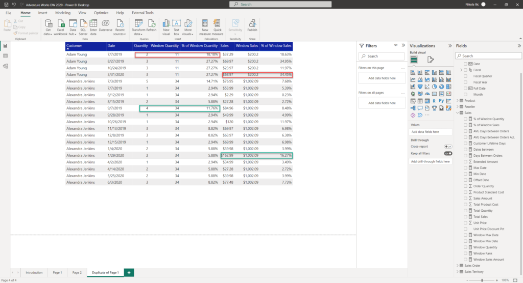
Now, we have a running total for each customer! So, we can for example now calculate a percentage of each individual purchase within the whole:

% of Window Quantity = DIVIDE([Total Quantity],[Window Quantity],0)

% of Window Sales = DIVIDE([Total Sales],[Window Sales Amount],0)

So far, so good! Let’s do some more cool stuff. First, I’ll calculate how many days passed between two consecutive orders. For that task, another DAX window function comes to the rescue: OFFSET. Essentially, I want to grab the date of the previous row and calculate the difference in days between the current row date and the previous row date:

Offset Date = CALCULATE(
                        MIN('Date'[Date]),
                        OFFSET(
                            -1,
                            SUMMARIZE(ALLSELECTED(Sales),Customer[Customer],'Date'[Date]),
                            ORDERBY('Date'[Date]),
                            KEEP,
                            PARTITIONBY(Customer[Customer])
                        )
                        )

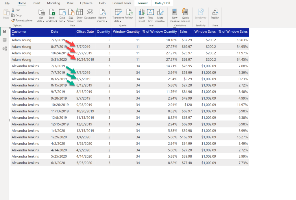
And, here is the measure to calculate the number of days between the orders:

Days Between Orders = DATEDIFF([Offset Date],MIN('Date'[Date]),DAY)

Ok, now, let’s calculate the average number of days between the orders for every customer:

AVG Days Between Orders = CALCULATE(AVERAGEX(
                  SUMMARIZE(
                            ALLSELECTED(Sales),Customer[Customer],'Date'[Date]),[Days Between Orders]),
                   WINDOW(
                        1,ABS,
                        -1,ABS,
                        SUMMARIZE(ALLSELECTED(Sales),Customer[Customer],'Date'[Date]),
                        ORDERBY ('Date'[Date]),
                        KEEP,
                        PARTITIONBY(Customer[Customer])
                   )
                   )

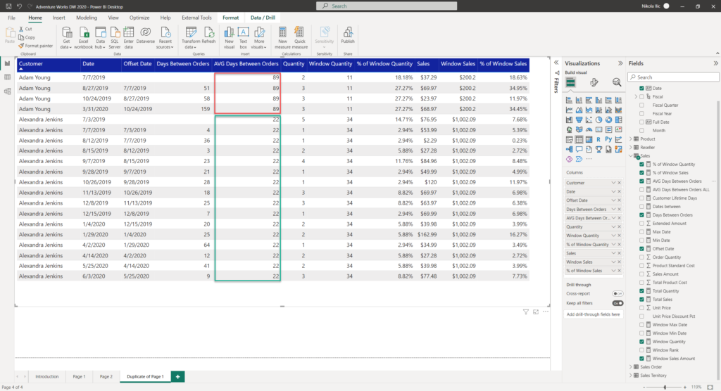
So, what can we conclude at this point? Alexandra orders on average every 22 days, while Adam needs 89 days on average to make a new order. How does that compare to a whole? Are 89 days way too long between the orders, or not?

So, let’s put these numbers into the context of the whole dataset.

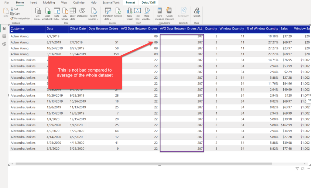
Although 89 days may look bad compared to 22 days for Alexandra Jenkins, we may conclude that these 89 days are not bad at all compared to the average for all the customers, which is 287 days! Great insight indeed!

Let’s wrap it up by calculating the total customer lifetime. This is the number of days between the first and the last order for each customer. So, let’s calculate the first and the last order date within our “windows”:

Window Min Date = CALCULATE(MIN('Date'[Date]),
                   WINDOW(
                        1,ABS,
                        -1,ABS,
                        SUMMARIZE(ALLSELECTED(Sales),Customer[Customer],'Date'[Date]),
                        ORDERBY ('Date'[Date]),
                        KEEP,
                        PARTITIONBY(Customer[Customer])
                   )
                   )

Window Max Date = CALCULATE(MAX('Date'[Date]),
                   WINDOW(
                        1,ABS,
                        -1,ABS,
                        SUMMARIZE(ALLSELECTED(Sales),Customer[Customer],'Date'[Date]),
                        ORDERBY ('Date'[Date]),
                        KEEP,
                        PARTITIONBY(Customer[Customer])
                   )
                   )

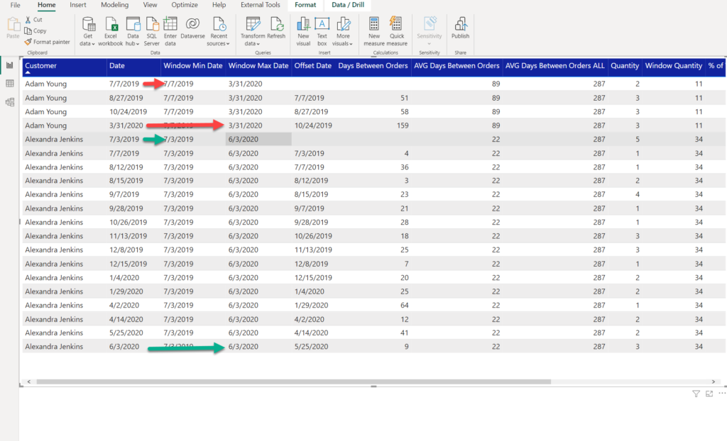
Here is the calculation for the number of customer lifetime days:

Customer Lifetime Days = DATEDIFF([Window Min Date],[Window Max Date],DAY)

And, once I drag it into the table, I can see that it’s being calculated within each window (for each customer separately):

Of course, this was just a basic example of what is possible by using DAX window functions. Honestly, there is an indefinite number of use cases to think of – for example, I could have also ranked individual rows within the window (and quickly identified the highest sales amount for each customer). I could have also partitioned by multiple attributes – for example, by customer AND month. Then, we would have a “window” containing all the rows for a customer within a single month. Think of it: Adam Young – July, Adam Young – August, Alexandra Jenkins – July, Alexandra Jenkins – August, and so on. Depending on your specific business request, your “window” can be defined differently.

Conclusion

Window functions are one of the most important enhancements to the DAX language, there is no doubt about that! Some of the business use cases that previously required writing complex and verbose DAX, now may be fulfilled in a more elegant and optimal way. Same as in SQL language, where window functions are one of the most powerful analytical tools, DAX window functions will definitely make many of the Power BI development tasks easier to implement.

Thanks for reading!

Last Updated on December 18, 2022 by Nikola

Spread the music: