
If you’ve been working with data platforms in recent years, chances are that you’ve implemented the medallion design pattern (or architecture:)) at least once. Bronze, silver, gold – raw, cleansed, curated – this design pattern has become so widely adopted that you’ll find it in every reference architecture, every certification exam, and every conference talk (including some of mine, I have to admit). And, in the vast majority of implementations I’ve seen (and built myself), all three layers are physically materialized as tables.
In this article, I’d like to challenge that habit. Not the medallion pattern itself – the logical separation of layers is, in my opinion, still of paramount importance. What I want to question is something much more specific: why is the silver layer a set of physical tables? And, with the recent announcement of GPU acceleration for the Fabric Data Warehouse, I believe this question deserves a serious answer, rather than “because that’s how the diagram looks”😀
For those of you who are new to the topic, a quick refresher before we proceed. In the medallion design pattern, the bronze layer stores raw data exactly as it arrived from the source systems, the silver layer contains cleansed and conformed data (deduplicated, standardized, validated), and the gold layer serves consumption-ready models, usually in the form of a star schema. Traditionally, each layer is persisted as delta tables, and pipelines move the data from one layer to the next.
An important disclaimer before we proceed…
The guidance in this article is based on my experience with implementing data platforms in real-world scenarios, combined with reasoning about what the new GPU-accelerated engine changes. Please bear in mind that this is not a “one size fits all” recommendation – quite the opposite, in fact. As you’ll see later in the article, there are scenarios where materializing the silver layer remains the right (and the only reasonable) choice. Therefore, you should always evaluate whether the approach proposed here makes sense in your specific use case. Consider it a general recommended practice for a certain class of workloads (I intentionally avoid the phrase best practice, because the “best” is very hard to determine and agree on), not a dogma to replace the old one.
Why did we materialize silver in the first place?
Let’s first take a step back and be fair to history, because materializing intermediate layers was not a mistake. It was a perfectly rational decision at the time when compute was the main bottleneck.
I’ve worked on various estates where transformation views were materialized for one simple reason: the appliance couldn’t efficiently handle a deep stack of layered views at query time. The query would spool out, the DBA would materialize the view, and everyone would move on with their lives. Then, these estates migrated to the cloud – Synapse dedicated pools, Redshift, GCP, Databricks, you name it – and the habit migrated with them, completely unchanged. Nobody re-evaluated the decision, because “staging, cleansed, consumption” was simply how a data warehouse looked.
To be precise, materializing the silver layer bought us four things:
- Query performance – transformations run once at load time, not on every read
- Compute isolation – heavy cleansing work doesn’t compete with BI queries
- A physical checkpoint – a durable snapshot of the “clean” data
- Incremental processing – tables allow us to process only what’s new, whereas views recompute everything
Now, here comes the interesting part. Points 3 and 4 are genuine architectural properties (please keep them in mind, as we’ll come back to them later. They define exactly where the approach proposed in this article breaks). However, points 1 and 2, which, in my experience, drive most materialization decisions in practice, are essentially a caching strategy. And caching strategies should be re-evaluated whenever the underlying hardware economics change.
Which brings us to the recent announcement…
What changed: GPU acceleration in Fabric Data Warehouse
Microsoft recently announced the GPU-accelerated Fabric Data Warehouse. Using NVIDIA accelerated computing, the engine takes the same T-SQL queries you know and love and executes them faster, especially, as stated in the announcement, when concurrency, scale, and complexity increase. The engineering behind it is documented in the CoddSpeed paper, which won the SIGMOD Best Industry Paper award, in case you want to go really deep into the internals.
From the practitioner’s point of view, the most important details are the following:
- There are no query rewrites and no new system to manage. You enable the feature from the workspace settings, and it applies to all SQL analytics endpoints and warehouses in that workspace (please remember this detail, as it has significant architectural implications, which we’ll discuss soon)
- The optimizer decides which portions of the query plan are eligible for GPU execution – operations like large joins and aggregations get pushed to GPUs, while the rest runs on CPUs. If a query is not eligible, it seamlessly runs on CPUs, preserving correctness
- Microsoft’s benchmarks against three comparable cloud data warehouse providers showed up to 7x faster performance. But, the number that caught my attention is a different one: at the 100 GB data scale, the full 22-query workload completed in approximately five seconds – regardless of whether one user or 64 concurrent users were running queries! Most data warehouses slow down and become less predictable as concurrency increases, so this stability under load is, in my opinion, the truly interesting part of the announcement
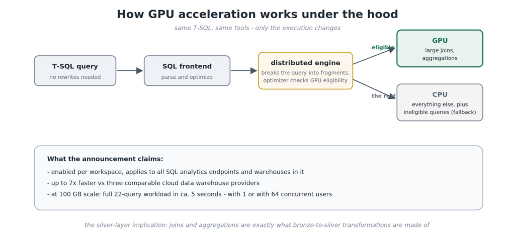
If we strip away the marketing buzz, the relevant claim is the following: the warehouse engine can now push joins and aggregations onto hardware that processes them massively in parallel. And, if you think about it for a moment, a typical bronze-to-silver transformation consists of… exactly these operations! Deduplication is a window function over a scan. Type conformance is a projection. Referential checks are joins. Standardizing country codes is a simple lookup. There is nothing exotic in the typical silver-layer logic – it’s deterministic, stateless work, and precisely the workload shape that the new engine accelerates.
Hence, the fair question would be: if the engine can execute your silver transformation logic over bronze data at query time, fast enough that nobody notices the difference, what exactly is the materialized silver table buying you?
I didn’t want to answer this question based on gut feeling, so I’ve prepared a benchmark, which we’ll examine later in this article. But first, let’s see how the proposed architecture looks.
The “virtualized” silver layer
The proposal fits in one sentence: keep bronze and gold materialized, and implement the silver layer as a schema of views.
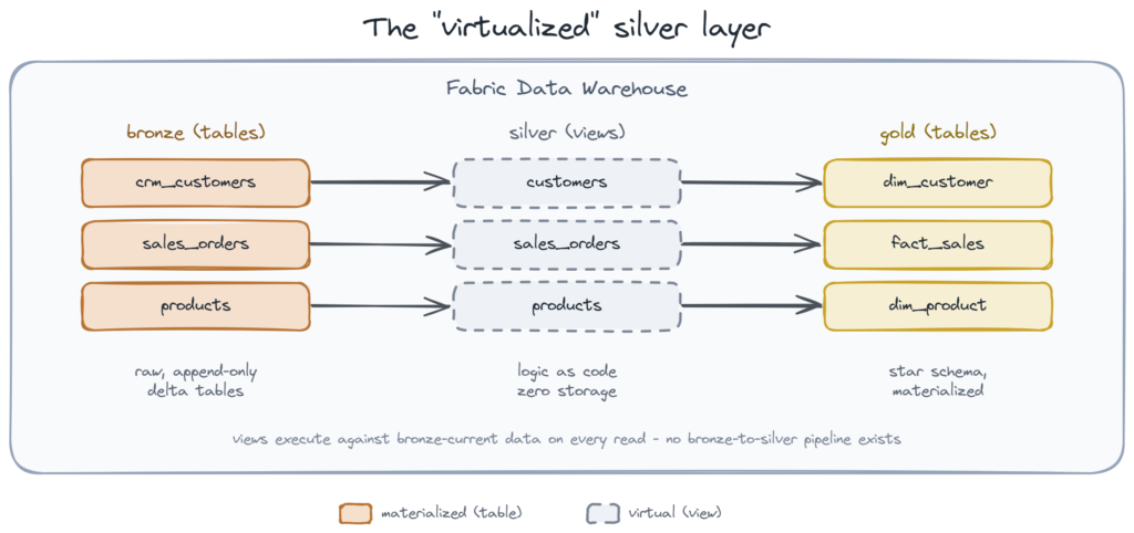
The bronze layer stays exactly what it should be – raw, append-only, the immutable record of what the source systems actually sent you. The gold layer also stays materialized, since BI concurrency and star schema performance still benefit from physical tables. The silver layer, however, becomes what it has always been logically: a set of transformation rules. The only difference is that these rules now live as view definitions, instead of being frozen into physical copies of the data.
Let’s illustrate this with a real-life example. Imagine the Meridian Bikes company (my usual demo “universe”), where the raw customer feed lands in bronze with all the usual mess: duplicates (the CRM sends full snapshots, and ingestion retries create extras), inconsistent country values (“AT”, “Austria”, “AUT” – all representing the same country, of course), and raw PII that we definitely don’t want floating around the analytical layer. The silver view handles all of it:
CREATE VIEW silver.customers AS
WITH deduplicated AS (
    SELECT
        *,
        ROW_NUMBER() OVER (
            PARTITION BY customer_business_key
            ORDER BY load_timestamp DESC
        ) AS rn
    FROM bronze.crm_customers
)
SELECT
    customer_business_key,
    TRIM(first_name)                          AS first_name,
    TRIM(last_name)                           AS last_name,
    -- PII masking happens in the view, not in a pipeline
    LEFT(email, 2) + '***@' +
        RIGHT(email, LEN(email) - CHARINDEX('@', email))
                                              AS email_masked,
    -- conform the country chaos to ISO codes
    CASE UPPER(TRIM(country_raw))
        WHEN 'AT'       THEN 'AT'
        WHEN 'AUT'      THEN 'AT'
        WHEN 'AUSTRIA'  THEN 'AT'
        WHEN 'DE'       THEN 'DE'
        WHEN 'GERMANY'  THEN 'DE'
        WHEN 'DEUTSCHLAND' THEN 'DE'
        ELSE 'UNKNOWN'
    END                                       AS country_code,
    city,
    load_timestamp
FROM deduplicated
WHERE rn = 1;
The sales feed brings its own flavor of chaos – European sources send the unit price as ‘1.249,99’, whereas American sources send ‘1249.99’, test orders pollute the stream, and ingestion retries duplicate the rows:
CREATE VIEW silver.sales_orders AS
WITH deduplicated AS (
    SELECT
        *,
        ROW_NUMBER() OVER (
            PARTITION BY order_id, source_system
            ORDER BY load_timestamp DESC
        ) AS rn
    FROM bronze.sales_orders
)
SELECT
    order_id,
    customer_business_key,
    product_id,
    CAST(order_date_raw AS DATE)              AS order_date,
    quantity,
    -- normalize the EU decimal format before casting
    CAST(
        REPLACE(REPLACE(unit_price_raw, '.', ''), ',', '.')
        AS DECIMAL(18,2)
    )                                         AS unit_price,
    source_system
FROM deduplicated
WHERE rn = 1
  AND is_test_order = 0;
And that’s the entire silver layer! No pipeline, no orchestration, no load to monitor. The gold refresh is a plain CTAS statement reading through the views, and the views execute against the current state of bronze every single time.
A point worth mentioning is the security aspect, which I consider underrated in this discussion. Row-level security and data masking sit naturally on views. The PII masking you saw above is not a separate governance pipeline that someone has to remember to run. It’s structurally impossible for the analytical layer to see the raw email address, because the raw email exists only in bronze, and bronze is locked down. In other words, views are not just a performance trade-off here – one might argue they represent a better governance boundary than tables.
What do you gain?
Let’s examine the benefits one by one.
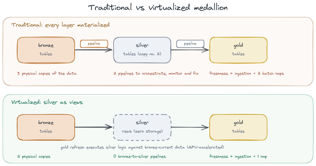
First and foremost, data freshness stops being an architecture problem. When gold refreshes, it reads through to whatever is in bronze at that very moment. The situation where “silver is four hours behind bronze” simply can’t occur, because there is no silver state to fall behind. I once sat in a meeting where an operations team asked, entirely reasonably, why their bookings dashboard lagged reality by half a day, and the honest answer was: “because of our architecture”. The ingestion was near-real-time, but the staleness was manufactured entirely by the layer-to-layer batch hops. The virtualized silver layer removes one of these hops from existence.
The second benefit is closely related to the first one: there is no bronze-to-silver pipeline to fail. Anyone who has ever been woken up by a failed overnight load (schema drift in one source table, silver stale, gold refreshed anyway, and the CFO looking at Tuesday’s numbers on a Thursday morning…) will appreciate this. The operational surface of the platform shrinks – fewer pipelines to orchestrate, monitor, and alert on.
Next, there is one fewer physical copy of the data. “Storage is relatively cheap nowadays”, I hear you moaning. And, I agree with that. However, the second copy also costs you in maintenance operations, in backup surface, and, maybe most importantly, in answering the audit question: “which of these three customer tables is the real one?”
Finally, the deployment velocity. In a materialized silver layer, a schema change means: alter the table, update the pipeline, backfill the history, coordinate the gold refresh, and hope that nothing reads the data mid-migration. I’ve watched a fairly simple column rename take two full sprints to propagate through materialized layers at one of my clients, with a change advisory board meeting in the middle of the process. The same change in a virtualized silver layer? An ALTER VIEW statement, deployed in seconds through your regular CI/CD process, applied to the entire history instantly, because the history is recomputed, not stored. The silver layer becomes what dbt practitioners have known for years: transformation logic is code, and code should be cheap to change.
Where this approach breaks (please read before dropping your silver tables!)
Now, the part that every experienced reader has been waiting to throw at me😀 There are four serious objections, and I’ll be honest with you – two of them are strong enough that, for parts of your data estate, the answer will remain: materialize.
Stateful transformations don’t virtualize
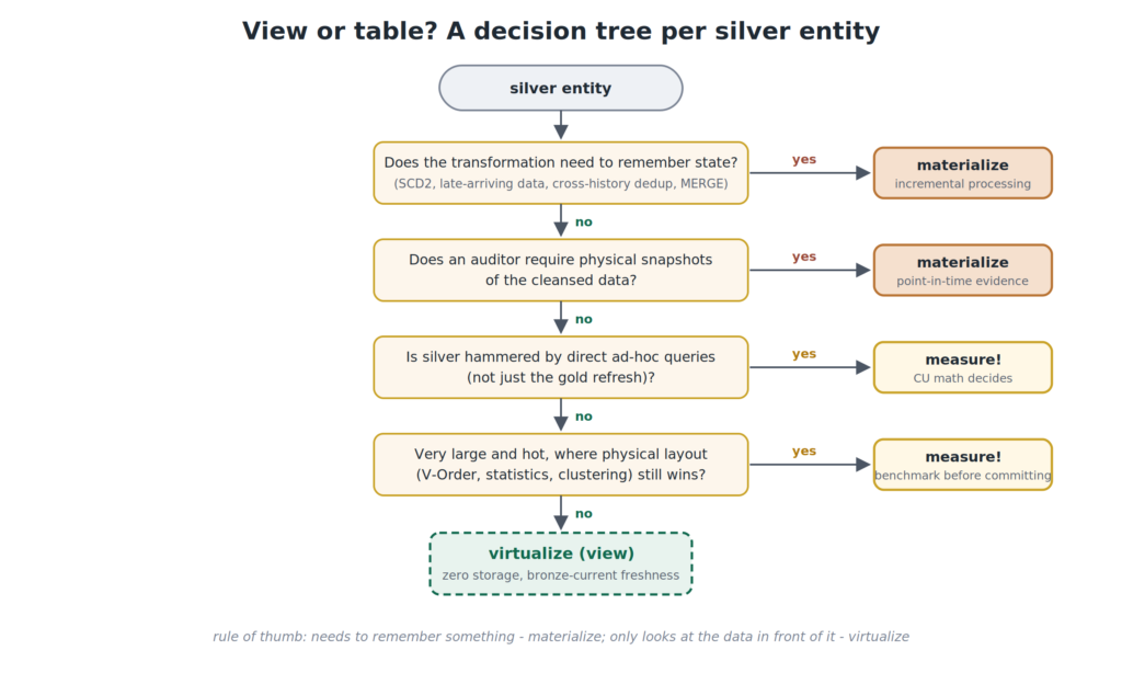
This is, without any doubt, the biggest one. A view recomputes its full logic on every execution. That works perfectly fine for stateless operations – deduplication within a snapshot, casting, conforming values. However, it doesn’t work for logic that depends on history: SCD Type 2 dimensions, late-arriving data handling, deduplication across years of accumulated records, or anything involving a MERGE statement.
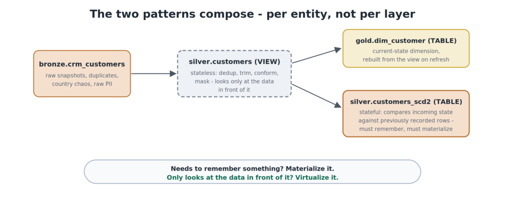
Let’s illustrate why. An SCD2 customer dimension needs to compare the incoming state against the previously recorded state, in order to close the old rows and open the new ones. The “previously recorded state” is, by definition, a materialized concept. A view would have to re-derive all validity intervals from the full bronze history on every single query, which is exactly the work that incremental processing exists to avoid. And no amount of GPU power changes the asymptotics of recomputing the entire history versus appending to it.
Therefore, the rule of thumb I’d suggest: if the transformation needs to remember something – materialize it! If it only looks at the data in front of it – virtualize it!
You give up physical optimization
V-Order, statistics, clustering, data layout in general – these are properties of materialized tables. A view over bronze inherits the physical layout of bronze, and there is nothing you can do about it. GPU acceleration compensates by brute-forcing the scan, but let’s be honest: “the hardware is fast enough to overcome my unoptimized layout” is a bet on hardware economics, not an engineering principle. For most silver-shaped workloads, this bet is perfectly fine. For your largest and hottest tables, please measure before you commit.
Reproducibility becomes conditional
With a materialized silver layer, answering the question “what did the cleansed data look like on March 3rd?” is a time-travel query. With a virtualized silver layer, the answer depends on two conditions: first, that your bronze retention covers March 3rd, and second, that your view logic is deterministic and versioned. Since the logic is code, it lives in Git, so you can reconstruct the exact transformation that was in effect on any given date. For most organizations, this is sufficient – one might even argue it’s cleaner, because logic changes are explicit commits rather than “invisible” pipeline edits.
However, and this is a big HOWEVER, if you operate in a regulated industry (banking, insurance, pharma…), an auditor may simply not accept “we re-ran the view” as evidence. They want the physical snapshot that a business decision was based on. Please make sure you know which world you live in, before architecting for the other one.
Direct silver consumers change the math
Everything we discussed so far assumes that the dominant read pattern is the gold refresh. In that case, silver views execute once per refresh cycle, and the compute economics are trivially in favor of views. However, if your data scientists query the silver layer directly, all day long, every single one of these queries re-executes the transformation logic against bronze.
Depending on the data volume and query frequency, this either doesn’t matter at all (GPU-accelerated scans over a few hundred gigabytes) or matters a lot (complex views over tens of terabytes, hit thousands of times per day). It’s worth mentioning that this objection is weaker than it used to be: the stability under concurrency that Microsoft demonstrated (the same ~5 second workload completion with 1 or 64 concurrent users) is precisely the scenario of many consumers hammering the same engine. Nevertheless, “stable under 64 users at 100 GB” is Microsoft’s benchmark, not yours – so the good news is that this is measurable, not philosophical. The benchmark scripts include exactly this ad-hoc pattern, so you can put your own numbers on it. And if your numbers say materialize, then materialize those specific entities, not the entire layer.
3, 2, 1… Let’s measure it!
Ok, enough theory! It’s time to challenge the assumptions with real numbers. I’ve prepared a set of scripts that you can run on your own Fabric capacity. Here is the scenario: our Meridian Bikes bronze layer contains ca. 500.000 customer records with an approximately 5% duplicate rate (and three different spellings of every country, obviously), plus ca. 10 million sales orders with roughly 2% duplicates, European decimal formats mixed with American ones, and around 1% test orders. In other words, everything you’d meet in real life, just reproducible.
The test builds the gold star schema twice: once reading through silver views, and once from materialized silver tables, measuring the end-to-end refresh time, the typical ad-hoc query patterns against silver itself, and the storage footprint.
An important note before we look at the numbers: I ran everything on my F4 capacity, on a tenant where GPU acceleration is not yet enabled (I asked Microsoft to enable GPU-accelerated queries on my tenant, but at the moment of writing, it’s still not enabled). Therefore, consider the results below the CPU baseline – the “before” picture. I will update this article with the “after” picture once the GPU-acceleration feature becomes available on my tenant, and that comparison will be the real test of this article’s thesis. In the meantime, the CPU numbers are interesting in their own right, as you’re about to see.
First, the end-to-end story, refreshing gold from freshly loaded bronze:
| Scenario | Silver as tables | Silver as views |
|---|---|---|
| Bronze-to-silver load | 25.9 s | 0 s (no load exists) |
| Gold refresh | 24.2 s | 31.7 s |
| End-to-end: fresh bronze to fresh gold | 50.2 s | 31.7 s |
| Silver storage footprint | 0.31 GB | 0 GB |
Let’s digest this. The gold refresh through views is indeed slower than the refresh from materialized tables (31.7 vs 24.2 seconds) – reading through the views re-executes the deduplication and casting logic, and that costs roughly 7 extra seconds. However, the views arm never pays for the bronze-to-silver load at all, so the complete cycle finishes 37% faster (31.7 vs 50.2 seconds) – on a plain F4, without any GPU in sight! The total CPU time tells the same story: ca. 75 CPU-seconds for the views arm vs ca. 103 for the tables arm per refresh cycle, which translates directly into capacity units you’re not burning. And the storage column speaks for itself: in my small demo, materializing silver added 0.31 GB – essentially a full second copy of the 0.32 GB bronze layer. The complete estate: 0.56 GB for the views arm vs 0.84 GB for the tables arm, or 50% more storage for the privilege of maintaining a pipeline.
Now, the ad-hoc queries against silver. And this is where I have to be honest with you, because the picture flips. Warm numbers are the median of 3 consecutive runs, whereas cold numbers come from a run executed right after a capacity pause/resume:
| Query | Views (warm) | Tables (warm) | Views (cold) | Tables (cold) |
|---|---|---|---|---|
| B1: aggregation (revenue by country and month) | 14.5 s | 3.7 s | 18.0 s | 3.9 s |
| B2: point lookup (one customer’s orders) | 15.2 s | 0.6 s | 15.3 s | 0.7 s |
| B3: wide scan (count and average by source) | 12.2 s | 0.1 s* | 12.5 s | 0.2 s* |
Three findings worth deepdiving here.
First, the aggregation penalty (B1) is roughly 4x on CPU – every ad-hoc query through the view re-executes the full transformation stack, and burns ca. 12x more CPU time doing it. This is exactly the workload the GPU announcement targets, so this ratio is the number I’m most curious to re-measure.
Second (and this one surprised me), the worst case is not the big aggregation, but the tiny point lookup (B2). Fetching one customer’s orders through the view took 15 seconds, a ca. 24x penalty, and longer than aggregating the entire table! The reason: the ROW_NUMBER() deduplication in the view blocks predicate pushdown, so the engine must execute the dedup over all 10.2 million rows before it can filter down to a single customer. If your users run selective queries against silver, dedup-style views are the pathological case – please keep this in mind.
Third, the asterisk on B3: the materialized table answered in under 200 milliseconds while scanning 0.06 MB of data – that’s not a scan, that’s the result cache doing its job. A fair reading is that materialized tables benefit from an additional caching layer that views over bronze can’t exploit in the same way (the first, uncached execution of B3 against the table took ca. 0.4 seconds – still ca. 29x faster than the view).
One more observation, as a bonus: the pause/resume penalty was surprisingly mild. The cold run came in only 5-25% slower than the warm medians across the board. The data lives in OneLake regardless, so a capacity restart doesn’t devastate performance the way a cache-dependent architecture would.
The takeaway from the CPU baseline: for the gold-refresh-dominant pattern, the virtualized silver layer already wins today, on regular CPU compute – faster end-to-end, fewer CPU-seconds, half the storage growth. For direct ad-hoc consumption of silver, the views tax is significant (4x on aggregations, 24x on selective lookups), and this is precisely the gap that GPU acceleration promises to close. Once the feature lands on my tenant, we’ll find out (and this section will get its “after” table).
Now, remember the detail I asked you to keep in mind earlier? GPU acceleration applies to all SQL analytics endpoints and warehouses in the workspace. This is not a footnote, it’s what makes the whole architecture practical. Since the acceleration covers the SQL analytics endpoint, your existing lakehouse bronze works as-is: the silver views in the warehouse can read the lakehouse delta tables through the endpoint, and still benefit from GPU execution. No need to relocate the bronze layer into the warehouse.
The decision matrix
As I mentioned in the disclaimer at the beginning – this is not a dogma, and “views vs. tables” is a per-entity decision, not a per-layer religion. Here is the matrix I’d suggest for evaluating each silver entity:
| Dimension | Favors views | Favors tables |
|---|---|---|
| Transformation type | Stateless: dedup within snapshot, casting, conforming, masking | Stateful: SCD2, late-arriving data, cross-history dedup, MERGE logic |
| Data volume | Small to large – GPU-accelerated scans absorb it | Very large and hot, where physical layout matters |
| Consumer pattern | Gold refresh is the dominant reader | Heavy direct ad-hoc access to silver |
| Freshness requirement | High – business wants bronze-current data | Relaxed – batch cadence is fine |
| Audit requirement | Logic-as-code reconstruction is acceptable | Regulator demands physical point-in-time snapshots |
| Change frequency | Logic evolves often, velocity matters | Logic is stable |
Based on the estates I’ve assessed over the years, my prediction is the following: roughly 70% of silver entities are stateless conforming logic that never needed to be tables, whereas roughly 30% genuinely earn their materialization. Hence, the right architecture for most organizations is a hybrid one. And the interesting realization is that this hybrid was always available, we just defaulted to 100% materialization, because that’s what the diagram showed us.
By the way, the two patterns compose nicely: in the demo scripts, the stateless silver.customers view feeds the stateful, materialized SCD2 dimension. Virtualized and materialized silver are not competing architectures – on the opposite, they complement each other, per entity.
This is where the industry is heading anyway…
In case the whole idea still sounds too contrarian, let’s zoom out for a moment. dbt has had ephemeral models (transformations that exist as logic and compile away into downstream queries) for years, and seasoned dbt practitioners routinely keep their staging models unmaterialized. Snowflake shops have been running view-heavy transformation stacks for a decade. And Databricks’ declarative pipelines are built on the idea that you declare the transformation, and the engine decides what to materialize, which is, in my opinion, the logical endgame of everything discussed in this article. Materialization is an optimization decision, and optimization decisions belong to the engine, informed by the actual workload – not to a diagram drawn before the first query ever ran.
And, before someone rightfully points it out in the comments: yes, Fabric already has its own answer to declarative pipelines – Materialized Lake Views! For those of you who haven’t played with them yet, an MLV lets you define a transformation as a declarative statement (in Spark SQL or PySpark), while Fabric handles the rest: it tracks dependencies between the views, orchestrates refreshes in the correct order, and enforces data quality constraints that you declare directly in the SQL definition. Moreover, a decision engine determines the optimal refresh strategy per run – incremental (processing only new or changed data, provided that you’ve enabled Change Data Feed on the source tables), full rebuild, or skipping the refresh entirely when nothing changed. Sounds familiar? It should, because this is exactly the “engine decides” philosophy we just discussed.
So, how does the approach proposed in this article relate to MLVs? I’d say they answer the same question from two different directions. MLVs automate materialization – you still get the physical copy of the data (it’s literally in the name), with the storage footprint and the refresh latency that come with it, but the engine takes over the orchestration and refresh decisions. The virtualized silver layer skips materialization – zero storage, bronze-current freshness, but the transformation cost moves to the read time. In addition, there is a practical split between the two: MLVs are a lakehouse/Spark feature, whereas the views proposed in this article live in the T-SQL world of the warehouse. Hence, depending on which engine your team calls home, Fabric now offers you two different ways to stop hand-crafting bronze-to-silver pipelines, and honestly, I consider that great news, regardless of which one you choose.
The GPU-accelerated Fabric warehouse doesn’t invent the “stop materializing everything by hand” idea. What it does is move the break-even point far enough that you can act on the idea manually, today, with plain T-SQL views, and win on a significant portion of your silver estate.
Conclusion
Although this article is by no means a definitive guide to virtualizing your silver layer, I sincerely hope it provides a solid starting point for questioning a pattern that most of us (me included) adopted without much questioning. The key takeaway I’d like you to remember: the medallion design pattern was never about physical layers – it was about logical contracts. Bronze promises raw fidelity, silver promises cleansed and trustworthy data, gold promises consumption-ready models. Nothing in these contracts says that each one must be a copy of the data on disk.
Again, it’s worth reminding that the approach proposed here relies on general recommended practices for a specific class of workloads – stateless, conforming transformations – and there will always be cases (SCD2, regulated industries, heavy direct silver consumption) where materializing remains the right choice. Evaluate per entity, measure on your own capacity, and let the numbers decide.
In one of the next articles, I plan to challenge the other rule: do you even need the bronze layer materialized? OneLake shortcuts would like a word…
Thanks for reading!
Thanks to Claude and Excalidraw for creating these nice-looking diagrams and visuals.
Last Updated on July 31, 2026 by Nikola


Ross Farrell
One implementation caveat that’s worth mentioning from real-world Fabric deployments.
If your Silver layer is virtualized using views or OneLake shortcuts, be careful not to treat it as a new security boundary.
Authorization follows the underlying objects, so a consumer querying a virtualized Silver object may still require permissions on the source Bronze data.
In practice this means the principle of least privilege extends all the way back to the root dataset unless you’ve deliberately materialized the data or introduced a genuine security boundary.
I actually ran into this with Gold Lakehouse shortcuts and downstream semantic models.
Even though users only had access to Gold, the shortcut preserved the lineage back to Silver, so users without Silver access couldn’t query the model.
It’s also worth noting that Bronze isn’t always immutable or append-only in production.
GDPR deletions, replay corrections, CDC reconciliation and ingestion fixes all introduce legitimate mutations, so some organisations deliberately materialize Silver to establish both a governance boundary and a reproducible business contract, rather than purely for performance.
Top content otherwise!