Power BI – How to fit 200 million rows in less than 1GB!

When you are dealing with technology, sometimes you need to accept the fact that there are certain limits – especially when it comes to resources available. And sometimes, maybe more often than not, business requests are such that it’s hard or almost impossible to implement within the current setup.

I’ve faced a quite challenging task recently – to migrate an SSAS Multidimensional solution to Power BI. The “issue” was that the client has Pro license (which means, 1 GB model size limit), and there were approximately 200 million rows in the fact table (and constantly growing)!

I knew at first sight that there is no way to accommodate 200 million rows in under 1 GB, no matter how narrow and optimized the table is! I’ve already written about the best practices for data model size optimization, but here it simply wouldn’t work.

Initial considerations

When I start thinking about the possible solutions, the first and most obvious idea was to use Power BI as a visualization tool only and just do a Live Connection to a SSAS cube. However, this solution comes with the serious limitations – the most noticable one, you can’t enrich your semantic model by writing report level measures – and that was one of the key client’s requests! Therefore, Live Connection was immediately discarded…

The second obvious solution was to use DirectQuery mode for getting the data into Power BI. Instead of SSAS Cube, Power BI will directly target fact and dimension tables from the data warehouse. Despite all its limitations, Direct Query looked like a completely legitimate (and the only possible) solution. And this was the best I can thought of…

…Until I found Phil Seamark’s blog post about filtered aggregations that opened a whole new perspective! This whole series on creative aggregations is awesome, but this specific concept was enlightening to me.

Filtered aggregations in a nutshell

I won’t go into details about the concept, as Phil explained that much better than I ever would. Essentially, the idea is to separate “hot” and “cold” data, and then leverage the Composite model feature in Power BI – importing the “hot” data in Power BI, while “cold” data will stay in the data warehouse and be targeted through Direct Query. On top of that, applying aggregations within the Power BI data model will bring even more benefit, as you will see later.

Now, I hope you are familiar with the terms “hot” and “cold” data – for those of you who are not – “hot” data is the most recent one, where word “recent” has typical “it depends” meaning. It can be data from last X minutes, hours, days, months, years, etc. depending on your specific use case.

In my case, after talking to report users, we’ve concluded that the most of the analysis focuses on the data from previous 3 months. Therefore, the idea is to extract “hot” data dynamically, as the data from 3 months prior to today’s date, and store that data in the Power BI tabular model. Report consumers will benefit from fast queries, as the data would be optimally compressed and kept in-memory. On the other hand, when older data is needed for analysis (“cold” data), Power BI will go directly to a data source and pull the data from there at the query time.

Finding the “tipping point” – the point in time to separate “hot” and “cold” data is of key importance here. If you opt to use a shorter period for “hot” data, you will benefit from having a smaller data model size (fewer data imported in Power BI), but you will have to live with more frequent Direct Query queries.

But, enough theory, let’s jump into Power BI Desktop and I will show you all the steps to fit your “200 million rows” fact table in less than 1 GB!

How it all started…

As you can see, my original fact table contains data about sport bets, and has around 200 million rows.

I also have two simple dimension tables – Date dimension and Sport Type dimension.

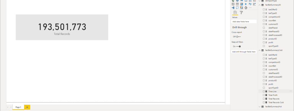
Since I’ve imported all the data in Power BI, I will check the metrics behind my data model. As you can see, pbix file size is slightly below 1 GB. And, this number increases on a daily level!

Let’s apply our first step and separate “hot” and “cold” data. You need to ensure that there is no overlapping between these two, but also no gaps in between, so you get a correct result in the end.

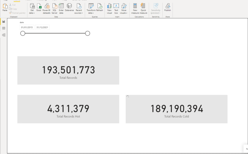
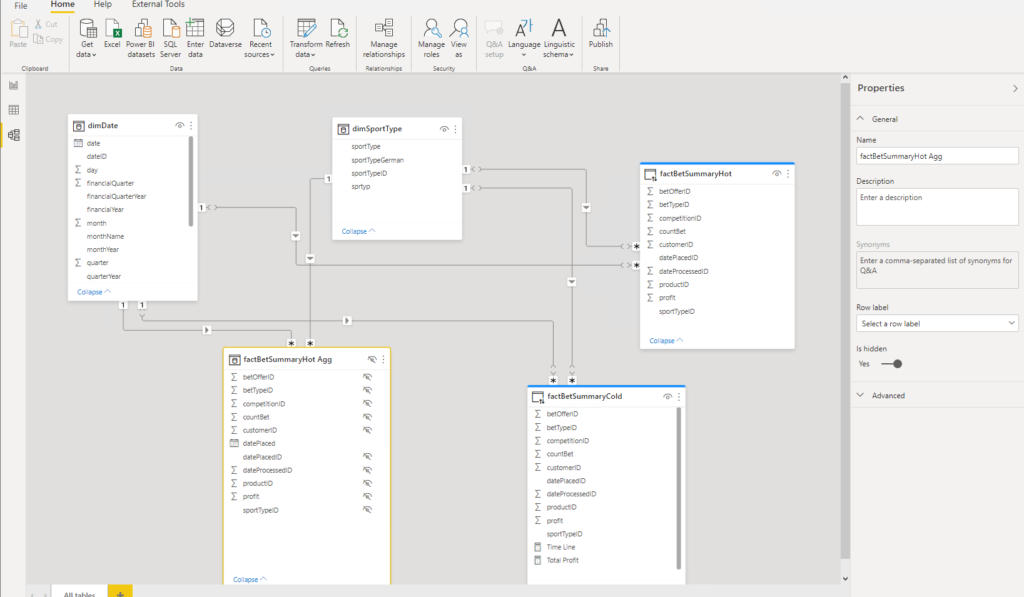
Here, we will leverage the Composite model feature within Power BI. I’ve splitted my giant fact table into two: factBetSummaryHot and factBetSummaryCold. The “hot” table will hold the data from the previous 3 calendar months, and in my case this table now has around 4.3 million rows.

I’ve started by creating both “hot” and “cold” tables in Direct Query storage mode. Then, I will first build an aggregated table over “hot” data and this table will use Import mode. On the other hand, the “cold” table contains the remaining ~190 million rows, and it will use Direct Query mode. On top of it, I will build a few aggregated tables to cover different dimension attributes (such as the date and sport type for example), and also use Import mode for these two aggregated tables, so Power BI will need to switch to Direct Query and target original data source only for those queries that are not satisfied with Import mode tables!

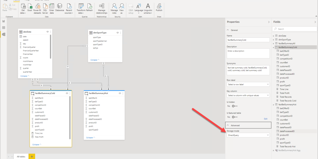
Ok, let’s now start implementing the filtered aggregation solution. I’ve switched the “cold” table to Direct Query storage mode, as you can see in the following illustration:

And, if I check the pbix file size now, I see that it’s only 17 MBs!

So, I achieved the starting request to fit the data in less than 1GB, as I managed to reduce the data model size from ~1GB GB to 17MB, while at the same time preserving the original data granularity!

Improving the original solution

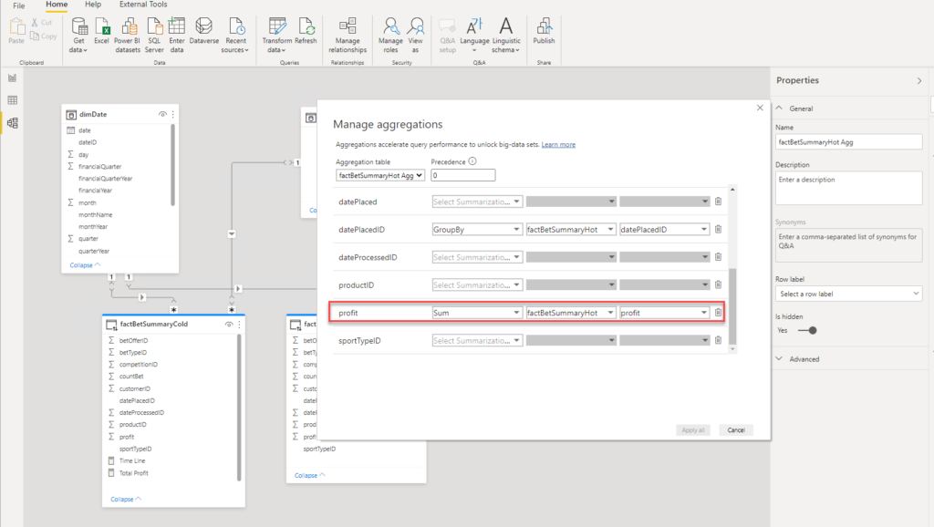
Now, let’s create an aggregated table over “hot” data, and set storage mode of this table to Import:

I will not go into detail about aggregations themselves, as there is an awesome article written by Shabnam Watson, where you can learn more about this powerful feature.

The next step is to establish relationships between newly created aggregated table and dimension tables:

Now, the performance of this report would depend on many things. If the user tries to interact with the report, and wants data older than 3 months, Power BI will go and search for that data through the ~190 million rows stored in the SQL Server database – having to cope with the network latency, concurrent requests, etc.

Let’s say that I want to analyze total profit, which is the simple SUM over Profit column. In order to retrieve the correct figure, I need to sum values from both “hot” and “cold” tables, writing the following DAX measure:

Total Profit Hot & Cold = 
                          VAR vProfitHot = SUM(factBetSummaryHot[profit]) 
                          VAR vProfitCold = SUM(factBetSummaryCold[profit])
RETURN
vProfitHot + vProfitCold 

Now, you would assume that if we want to see only the data from the previous 3 months, Power BI will go only to an aggregated table and quickly pull the data and render the visual for us. WRONG!

The following illustration shows that, despite selected dates are between January 31st and March 30th, Power BI needed almost 12 seconds to get my data ready! And, if we take a look at Performance Analyzer numbers, you will see that Direct Query took almost the whole part of that time:

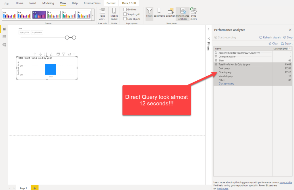
Why on Earth, Power BI needed to apply Direct Query, when we have our nice little aggregated table for this portion of the data? Well, Power BI is smart. In fact, it is very smart! It was smart enough to internally translate our SUM over profit column and hit the aggregation table, instead of “visiting” its Direct Query twin. However, there are certain situations when it can’t resolve everything on its own. In this scenario, Power BI went down and pulled all the data, even from the “cold” Direct Query table, and then applied date filters!

That means, we need to “instruct” Power BI to evaluate date filters BEFORE the data retrieval! And, again, thanks to Phil Seamark for the improved version of the measure:)

The first step is to set the “tipping point” in time in DAX. We can do this using exactly the same logic as in SQL, when we were splitting our giant fact table into “hot” and “cold”:

Time Line = 
           VAR maxDate = CALCULATE(
                                 MAX('factBetSummaryHot Agg'[datePlaced]),
                                 ALL()
                                  )
RETURN 
    EOMONTH(DATE(YEAR(maxDate),MONTH(maxDate)-3,1),0)

This measure will return the cut off date between the “hot” and “cold” data. And, then we will use this result in the improved version of Total Profit measure:

Total Profit = 
               VAR vProfitHot = SUM(factBetSummaryHot[profit])
               VAR vProfitCold = IF(
                                     MIN(dimDate[date]) < [Time Line] ,
                                     SUM(factBetSummaryCold[profit])
                                   )
RETURN
vProfitHot + vProfitCold
    

Here, we are in every scenario returning SUM over profit column from the “hot” table, as it will always hit the aggregated table in Import mode. Then, we are adding some logic to “cold” data – checking whether the starting date in the date slicer is before our “tipping point” – if yes, then we will need to wait for the Direct Query.

But, if not, well…

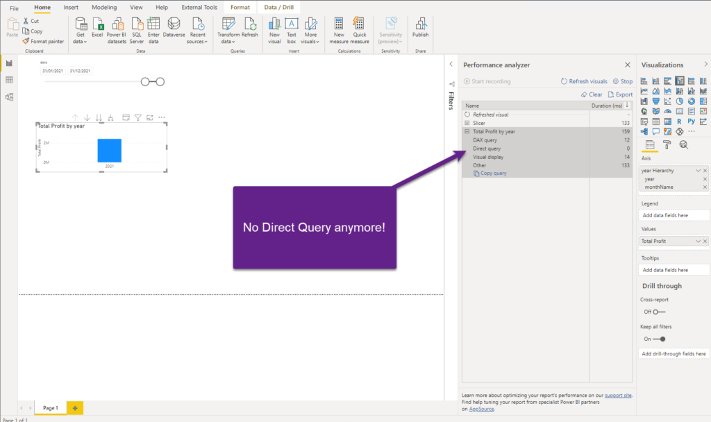
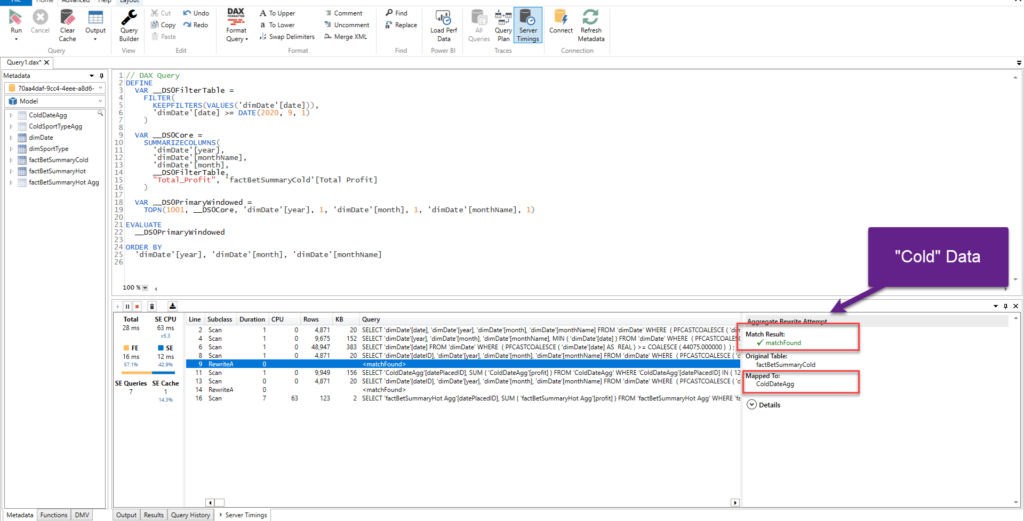
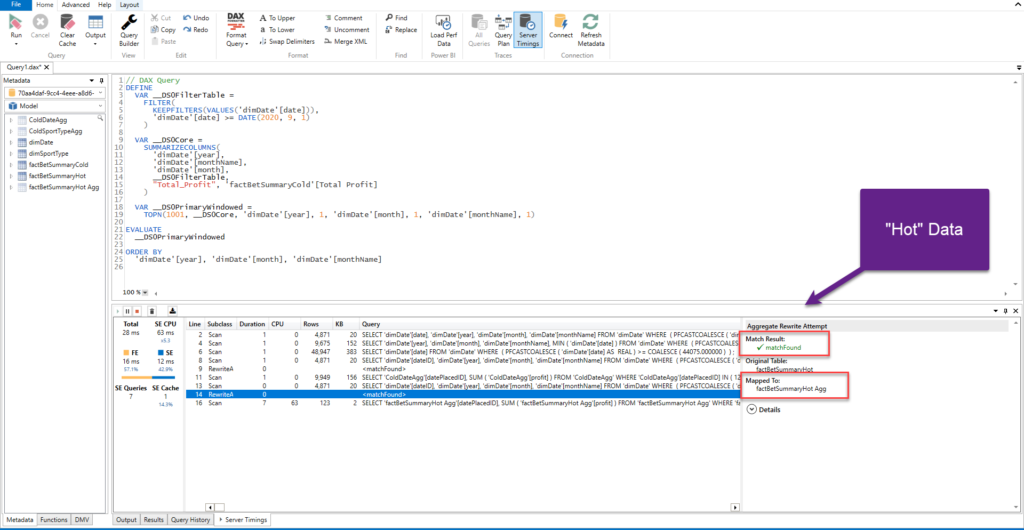
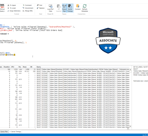
As you can see, now we got our visual displayed in 159 milliseconds! And, the DAX query took 12 milliseconds! No Direct Query this time, and if we go and check the query in DAX Studio, we will notice that our aggregation table was matched, even if we used the Direct Query table as a reference within the measure!

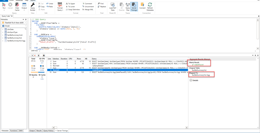
That’s fine, as it means that most frequently running queries (targeting data from the previous 3 months) will be satisfied using the Import mode aggregated table!

Handling “cold” data

As the next optimization step, I want to build an aggregated tables over “cold” data, that could potentially satisfy the most frequently ran users’ queries, which need to pull the data before the “tipping point” (older than 3 months). That will slightly increase the data model size, but it will significantly increase the report performance.

So, only in some specific use cases, when a user needs to see some low level of grain within the “cold” data, Power BI will fire the query directly to an underlying database.

Let’s create two aggregated tables over “cold” data, based on our dimensions. The first will aggregate the data based on the date:

SELECT datePlacedID
      ,SUM(profit) profit
      ,SUM(countBet) countBet
FROM factBetSummaryCold
GROUP BY datePlacedID

While the second will aggregate the data grouped by sport type:

SELECT sportTypeID
      ,SUM(profit) profit
      ,SUM(countBet) countBet
FROM factBetSummaryCold
GROUP BY sportTypeID

Let’s build relationships between these two aggregated tables and our dimensions and set aggregations for our newly imported tables:

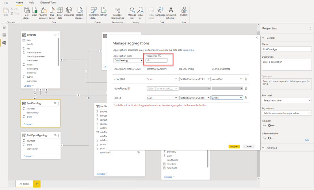
By setting the Precedence property, you can “instruct” Power BI which aggregated tables to use first. The higher the Precedence value, the higher priority gets respective table.

Let’s go back to our report and check the performance of our measure once we include the data from before the “tipping point”:

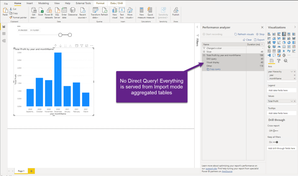
Awesome! I’ve expanded the date range to the previous 6 months and we got our results back in 198 milliseconds, while the DAX query took only 40 milliseconds! If we take a deeper look in DAX Studio, we can confirm that both “parts” of our request, for both “cold” and “hot” data, were served from Import mode aggregated tables:

Before we draw a conclusion, let’s take a final look to our pbix file size:

That’s incredible: 18MB!

Conclusion

As you witnessed, we made it! The original request was to move a data model from SSAS cube to Power BI Pro workspace, without losing any of 200 million rows from the fact table! We started at almost 1GB and finished at 18MB, while preserving original data granularity, and without impacting the report performance for 99% of use cases!

Extraordinary tasks require extraordinary solutions – and, if you ask me, thanks to Phil Seamark’s brilliant idea – we have a solution to accommodate extremely large data even into Pro limits.

Essentially, what we’ve just done is that we’ve managed to fit 200 million rows in 18MB…

Thanks for reading!

Last Updated on July 20, 2021 by Nikola