CLUSTER BY in Fabric Warehouse: when the magic shows up and when it doesn’t!

Last week, I was reviewing a Fabric Warehouse with one of my clients. The classic data warehouse setup – a fact table sitting at around 800 million rows, a Power BI report on top doing aggregations by country and date, and a complaint from the business team: “The report is slow.”

The first thing every Fabric architect reaches for in this situation is the usual playlist: check the query plan, look at the joins, validate the statistics, maybe scale up the capacity. All worth doing, but none of those things addressed what was actually happening: the warehouse was scanning the entire table for every filtered query, because there was no way to tell it which Parquet files actually contained the rows we cared about.

However, Microsoft shipped data clustering in preview at the end of November 2025, and the entire conversation changed.

In this article, I want to walk you through what data clustering is, how it works under the hood, and most importantly, I’ll show you a real demo on a 100-million-row clickstream table that you can run in your own warehouse. No abstractions, no marketing numbers, but actual T-SQL you can paste.

Let’s get into it.

What is data clustering, really?

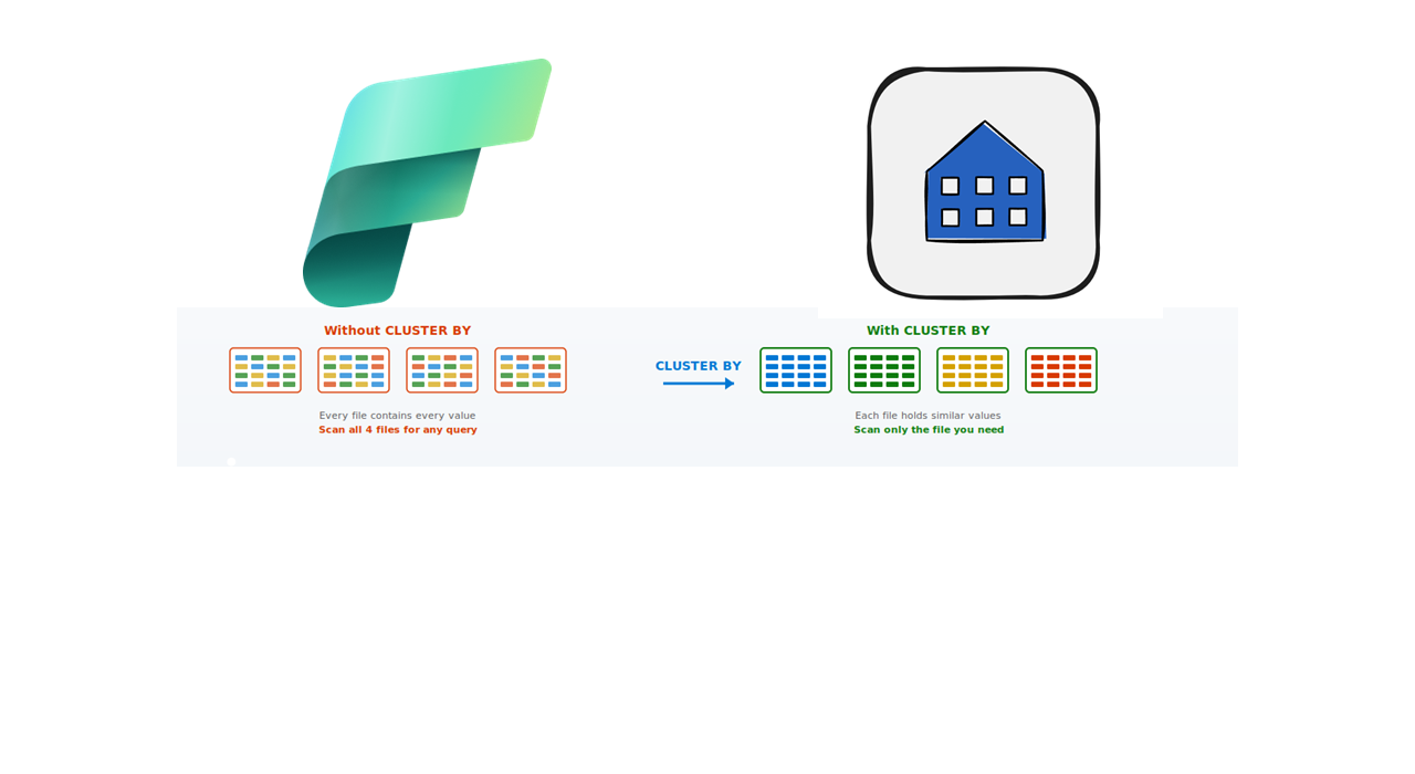
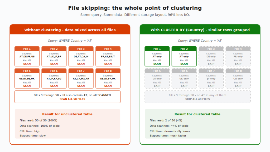
Data clustering is a technique that organizes rows in storage based on similarity. Rows with similar values across one or more chosen columns are physically stored close together in the underlying Parquet files. When you later run a query with a WHERE clause on those columns, the warehouse engine can read the file metadata, see that most files don’t contain any matching rows, and skip them entirely.

And, that’s the whole idea:)

But let me introduce the part that took me some time and thinking to fully appreciate: data clustering in Fabric Warehouse is NOT the same thing as a traditional clustered index. A clustered index in SQL Server uses lexicographical ordering. This means, row A comes before row B because that’s the dictionary order. Fabric’s clustering algorithm uses a space-filling curve to preserve locality across multiple dimensions at once. Which means if you cluster by, say, Country and EventDate, the engine can keep rows close together that have similar values on BOTH columns, not just sort by one and then the other.

I hear you, I hear you: Nikola, what on Earth is a “space-filling curve”? What does it actually mean for me? In practice, it means you can cluster by up to four columns, and the engine treats them as a unit, not as a sort priority. The order you specify the columns in doesn’t matter, which is the most counterintuitive part for anyone coming from a traditional indexing background.

The big takeaway from this diagram: clustering doesn’t make your storage smaller, and it doesn’t make individual file reads faster. It just makes the engine smarter about which files it bothers to read in the first place.

How clustering works during ingestion

There are some very interesting points about clustering, from an architect’s perspective.

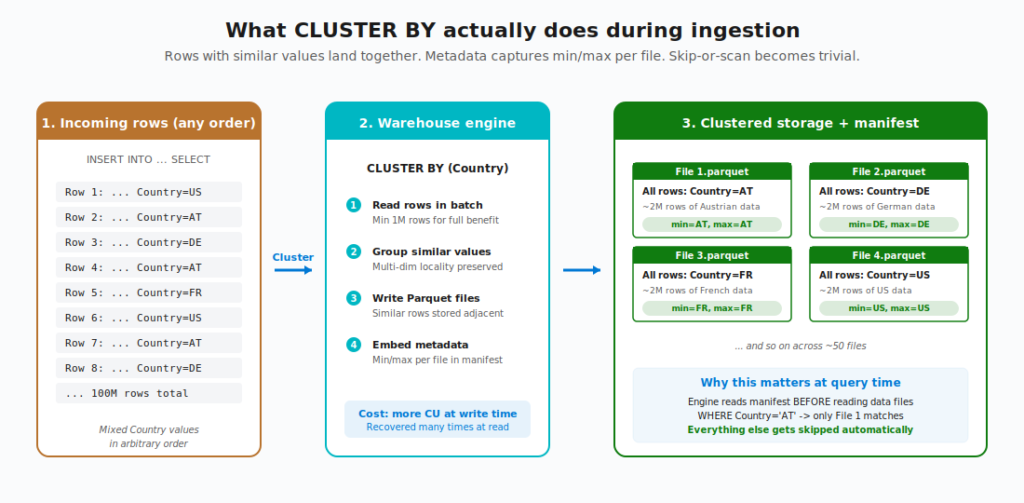
When you INSERT INTO a clustered table (or use CREATE TABLE AS SELECT), the warehouse engine reads your incoming rows in batch, applies the clustering algorithm to figure out where each row should land, and writes Parquet files where similar values are physically adjacent. During this process, it also embeds metadata into the file manifest – things like min and max values per column, per file. That manifest is the magic ingredient.

A few things worth flagging here:

You pay at write time, you get paid back at read time. Clustering adds overhead to ingestion, because the engine has to do extra work to figure out the right layout. Microsoft’s docs are explicit about this: “Data ingestion incurs more time and capacity units (CU) on a table that uses data clustering when compared with an equivalent table with the same data without data clustering.” So if your data is written once and read 50 times by reports, this is a well-worth trade-off. If your data is written once and read once, it’s probably not.

Batch size matters. Clustering works best when you ingest at least 1 million rows at a time. Smaller batches may trigger asynchronous reorganization (the engine compacts smaller files in the background), and the table might not be fully optimized immediately after ingestion. For batch ETL workloads, this is fine, as the next query that hits the table will benefit. For trickle inserts of a few hundred rows, you won’t see much.

You can’t add clustering to an existing table. This one is important to remember. CLUSTER BY must be defined at table creation. You can’t ALTER TABLE ... ADD CLUSTERING. If you want to add clustering to an existing table, your only option is to use CREATE TABLE AS SELECT to create a new clustered copy and rename. Hence, plan ahead.

When should you use CLUSTER BY?

Not every table benefits from clustering. In fact, most small or rarely-filtered tables will be worse off if you add it. Here’s the decision tree I use when reviewing client warehouses:

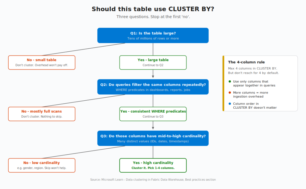
Let me unpack each question.

“Is the table large?” Clustering’s whole value proposition is file skipping. If your table fits in a handful of files anyway, there’s not much to skip. As a rough guide, tables under 10 million rows rarely show meaningful gains. Tables with hundreds of millions or billions of rows benefit dramatically. The bigger the table, the bigger the win.

“Do queries repeatedly filter the same columns?” Clustering helps WHERE predicates. If your workload is mostly full table scans, aggregations across the whole dataset, or filters on columns that change every time – clustering doesn’t help. The sweet spot is reports, scheduled reports, and recurring queries that always filter on the same handful of columns.

“Do those columns have mid-to-high cardinality?” This is where most people get it wrong. Clustering by Gender (2-3 distinct values) or Region (5-10 distinct values) won’t help much because those values are inherently spread across many files. Clustering by CustomerID (millions of distinct values) or EventDate (thousands of distinct values) gives the engine real opportunities to colocate similar values into specific files and skip everything else.

One more rule worth remembering: you can use up to four columns in CLUSTER BY, but don’t reach for four by default. Use only the columns that actually appear together in your query predicates. More clustering columns means more ingestion overhead, and the benefit only materializes if your queries use all of them. As Microsoft’s documentation puts it: “Multi-column clustering adds complexity to storage, adds overhead, and might not offer benefits unless all the columns are used together in queries with predicates.”

OK, theory’s done. Let me show you what this looks like with real numbers.

The demo: 100 million clickstream rows

For this walkthrough, I’m going to build a realistic web analytics scenario. Imagine you run a busy SaaS product and you’re collecting clickstream events – every page view, every interaction, every user session. Over time, you accumulate hundreds of millions of events. Your analytics team wants to query this data daily to investigate user behavior by country, by date, by page.

The table looks like this:

Column	Type	Cardinality
EventID	BIGINT	100M distinct (every row)
SessionID	BIGINT	~10M distinct
UserID	INT	~1M distinct
EventTime	DATETIME2	~hundreds of thousands distinct
EventDate	DATE	~365 distinct
PageID	INT	~5,000 distinct
Country	VARCHAR(2)	~200 distinct

Three of these columns are excellent clustering candidates: EventDate, Country, and PageID. They’re all mid-to-high cardinality, and they’re the ones the analytics team filters on every day. Let’s see what happens.

Step 1: Create the warehouse and the unclustered baseline

First, the unclustered version:

-- Create the baseline (unclustered) table
CREATE TABLE dbo.clickstream_unclustered (
    EventID BIGINT NOT NULL,
    SessionID BIGINT NOT NULL,
    UserID INT NOT NULL,
    EventTime DATETIME2(0) NOT NULL,
    EventDate DATE NOT NULL,
    PageID INT NOT NULL,
    Country VARCHAR(2) NOT NULL
);

Nothing fancy here, just a regular Fabric warehouse table.

Step 2: Generate 100 million rows

This is the part most articles skip. They tell you “imagine you have a large table” and leave you to figure out the rest. Let’s actually build one. A word of warning for all of you coming from a traditional SQL Server background: you can’t generate large datasets directly from system catalog views like sys.all_columns. If you try, you’ll get an unhelpful error: “The query references an object that is not supported in distributed processing mode.” This is by design – Fabric Warehouse can’t mix system catalog data with user data in distributed writes. Thanks to Koen Verbeeck for documenting this gotcha clearly on his blog.

The workaround is a two-stage approach: build a Numbers table as a regular user table first, then use it as the source for the synthetic data INSERT.

-- Seed table with digits 0-9
CREATE TABLE dbo.Digits (d INT NOT NULL);
INSERT INTO dbo.Digits VALUES (0),(1),(2),(3),(4),(5),(6),(7),(8),(9);

-- Numbers table: 10^8 = 100,000,000 rows via cross-joined digits
CREATE TABLE dbo.Numbers (n BIGINT NOT NULL);

INSERT INTO dbo.Numbers (n)
SELECT 
    d1.d + d2.d * 10 + d3.d * 100 + d4.d * 1000 
    + d5.d * 10000 + d6.d * 100000 + d7.d * 1000000 + d8.d * 10000000 + 1 AS n
FROM dbo.Digits d1
CROSS JOIN dbo.Digits d2 CROSS JOIN dbo.Digits d3 CROSS JOIN dbo.Digits d4
CROSS JOIN dbo.Digits d5 CROSS JOIN dbo.Digits d6 CROSS JOIN dbo.Digits d7
CROSS JOIN dbo.Digits d8;

This creates a regular user-owned table with 100 million sequential integers. Build it once, reuse it for any data generation work going forward. It’s worth keeping around.

Now, let’s populate the clickstream table from numbers:

INSERT INTO dbo.clickstream_unclustered
SELECT 
    n AS EventID,
    (n % 10000000) + 1 AS SessionID,
    (n % 1000000) + 1 AS UserID,
    DATEADD(SECOND, n % 31536000, '2025-01-01') AS EventTime,
    CAST(DATEADD(SECOND, n % 31536000, '2025-01-01') AS DATE) AS EventDate,
    (n % 5000) + 1 AS PageID,
    CASE n % 200
        WHEN 0 THEN 'AT' WHEN 1 THEN 'DE' WHEN 2 THEN 'FR'
        WHEN 3 THEN 'US' WHEN 4 THEN 'UK' WHEN 5 THEN 'IT'
        WHEN 6 THEN 'ES' WHEN 7 THEN 'NL' WHEN 8 THEN 'BE'
        WHEN 9 THEN 'PL' WHEN 10 THEN 'CZ'
        ELSE CHAR(65 + (n % 26)) + CHAR(65 + ((n / 26) % 26))
    END AS Country
FROM dbo.Numbers;

A few notes on this script:

• The two-stage pattern (Digits -> Numbers -> target table) is the bulletproof approach in Fabric Warehouse. The intermediate Numbers table is a regular user table, so it can be cross-joined and filtered freely without hitting the distributed-processing limitation.
• I’m using modular arithmetic (n % N) to spread values, which gives you uniformly distributed data. Real clickstream is usually skewed (some countries dominate, some pages are visited more), but this is close enough for the demo.
• The CASE expression for Country puts the well-known countries first, so the demo query WHERE Country = 'AT' returns a clean ~500K rows. The rest get random two-letter codes for variety.
• On my F64 Trial capacity, the 100M-row INSERT took less than a minute (50 seconds, to be more precise).
• If the single-shot 100M INSERT is unstable on your capacity, chunk it into 10M-row batches with a WHERE n > @start AND n <= @end filter on Numbers.

Step 3: Create the clustered version

Now the interesting bit. Same data, but with CLUSTER BY:

-- Create the clustered version using CTAS
CREATE TABLE dbo.clickstream_clustered 
WITH (CLUSTER BY (Country, EventDate, PageID))
AS 
SELECT * FROM dbo.clickstream_unclustered;

That’s the whole thing – one WITH clause! Same table structure, same 100M rows, but now clustered by the three columns that actually matter for our analytics workload.

Note that I picked three columns, not four. Country for the geo filter, EventDate for the time range filter, PageID for the page-level analysis. I deliberately did NOT add UserID even though it has high cardinality, because the dashboard queries we care about don’t filter by user. So, adding it would only add ingestion overhead with no payoff.

Creating and populating a clustered twin took 52 seconds on my F64 Trial capacity, so basically, there was no difference compared to the nonclustered version.

Step 4: Run the same query against both tables

Here’s the test query. A realistic analytics workload – “show me activity for Austria in November 2025”:

-- Against the unclustered table
SELECT 
    'Unclustered' AS label,
    EventDate,
    PageID,
    COUNT(*) AS event_count,
    COUNT(DISTINCT UserID) AS unique_users
FROM dbo.clickstream_unclustered
WHERE Country = 'AT'
  AND EventDate >= '2025-11-01' 
  AND EventDate <  '2025-12-01'
GROUP BY EventDate, PageID
OPTION (LABEL = 'Unclustered');

-- Against the clustered table
SELECT 
    'Clustered' AS label,
    EventDate,
    PageID,
    COUNT(*) AS event_count,
    COUNT(DISTINCT UserID) AS unique_users
FROM dbo.clickstream_clustered
WHERE Country = 'AT'
  AND EventDate >= '2025-11-01' 
  AND EventDate <  '2025-12-01'
GROUP BY EventDate, PageID
OPTION (LABEL = 'Clustered');

The OPTION (LABEL = ...) is the secret ingredient here. It tags each query with a custom label that we can later filter on in Query Insights.

Step 5: Compare the results in Query Insights

After running both queries, head to Query Insights (hint. wait for a few moments for query details to actually appear in the queryinsights schema) and compare:

SELECT 
    label,
    row_count,
    total_elapsed_time_ms,
    allocated_cpu_time_ms,
    data_scanned_disk_mb + data_scanned_memory_mb + data_scanned_remote_storage_mb 
        AS total_data_scanned_mb
FROM queryinsights.exec_requests_history
WHERE label IN ('Unclustered','Clustered')
ORDER BY submit_time DESC;

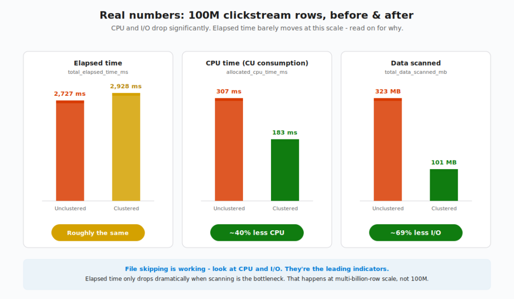
In my demo run on F64 Trial capacity, here’s what the numbers looked like:

Now this is where I want to be honest with you, because the result is more nuanced than the announcement blog might lead you to expect.

Look at the three metrics:

• CPU time: 307 ms vs 183 ms. The clustered version used about 40% less CPU. That’s real, that’s measurable, and it directly translates to less capacity unit (CU) consumption on your bill.
• Data scanned: 323 MB vs 101 MB. The clustered version read about 69% less data from storage. Again, real and measurable. This is file skipping working exactly as designed.
• Elapsed time: 2,727 ms vs 2,928 ms. Almost identical and within the noise margin. The clustered version was technically slower by 200 ms in this particular run.

Did I just write 3,000 words to tell you that clustering didn’t make the query faster?

No! I want to walk you through what’s actually happening, because this is one of those moments where the metrics tell a story that “X times faster” headlines don’t capture.

The mechanism is working perfectly. The 69% reduction in data scanned proves it. The engine is reading the manifest, identifying files that don’t contain Country = 'AT', and skipping them. The 40% CPU reduction is the direct consequence – less data to read means less CPU to process it. These savings are real, and they show up in your bill.

So why isn’t elapsed time also down 40-69%? Because at this query size, elapsed time isn’t dominated by data scanning. It’s dominated by fixed-cost overhead: query parsing, distributed execution coordination, statistics evaluation, result set marshaling, and network round-trip. These costs exist regardless of how much data you scan. When the underlying work takes ~200 ms instead of ~600 ms, the savings get absorbed by the overhead that takes another ~2,500 ms either way.

Where does the elapsed-time benefit show up? When the table is large enough that scanning IS the bottleneck. Microsoft’s announcement post benchmarked clustering on a 60-billion-row, 1 TB table – 600x bigger than my 100M-row demo – and reported 24x elapsed-time speedup with 65x less CPU and only 3.7% of data scanned. At that scale, the I/O reduction becomes the dominant factor, and elapsed time tracks it. At my 100M-row scale, the I/O reduction is real, but it’s not enough to overwhelm the fixed overhead.

This is actually one of the most useful things you can learn about clustering, and almost nobody talks about it. The leading indicators that file skipping is working are CPU and data scanned. Elapsed time follows, but it only follows dramatically when the workload is truly I/O-bound.

So what should you take away from this demo?

If you have a 100M-row fact table that’s already querying in under 3 seconds, clustering will save you CPU and capacity consumption, but it won’t make your report feel faster to users. The reports already feel responsive.

If you have a multi-billion-row fact table where queries currently take 30+ seconds, clustering is going to be a game-changer. The I/O reduction will be the dominant cost, the elapsed-time gains will be dramatic, and your users WILL notice.

In other words: clustering is most valuable on tables that are slow because they’re big, not on tables that are slow because of complex logic. Know which problem you have before you reach for clustering.

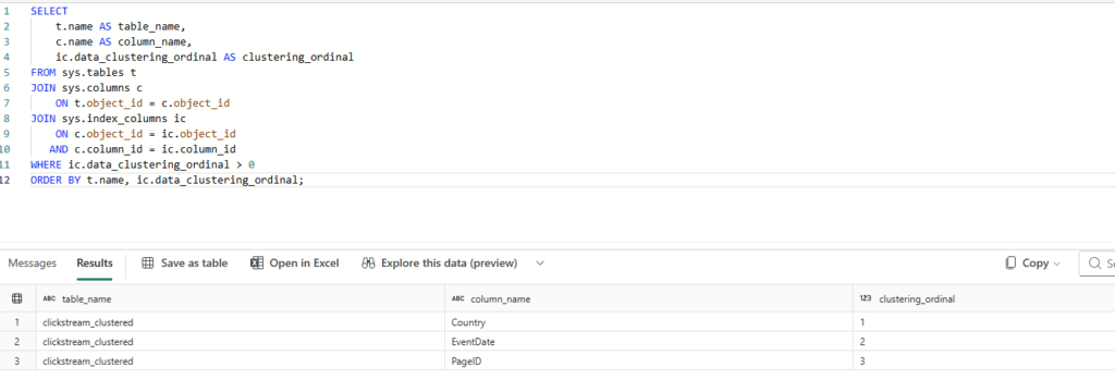
Verifying clustering is actually working

After you create a clustered table, you can verify it’s set up correctly by querying sys.index_columns:

SELECT
    t.name AS table_name,
    c.name AS column_name,
    ic.data_clustering_ordinal AS clustering_ordinal
FROM sys.tables t
JOIN sys.columns c
    ON t.object_id = c.object_id
JOIN sys.index_columns ic
    ON c.object_id = ic.object_id
   AND c.column_id = ic.column_id
WHERE ic.data_clustering_ordinal > 0
ORDER BY t.name, ic.data_clustering_ordinal;

You’ll see one row per clustering column, with clustering_ordinal indicating the position in the CLUSTER BY clause. Quick reminder from earlier: the column order doesn’t affect performance, it’s only displayed for reference.

The fine print: limitations and caveats

Like any feature in preview, clustering has rough edges. Here are some of the things I learned the hard way (so you don’t have to):

You can’t change clustering columns after the fact. As mentioned earlier, CLUSTER BY is defined at table creation and can’t be modified. If you need to change the clustering columns, you’re CTAS-ing into a new table.

SELECT INTO doesn’t support clustering. Only CREATE TABLE and CREATE TABLE AS SELECT accept the CLUSTER BY clause. If your existing pipelines use SELECT INTO patterns, you’ll need to refactor.

Data types matter. Not every column type can be used in CLUSTER BY. The big ones to avoid: bit, varchar(max), varbinary(max), and uniqueidentifier. Most of your candidate columns – integers, dates, regular varchars – work fine. For varchar columns, only the first 32 characters are used in column statistics, so clustering on a column with long shared prefixes (think URLs that all start with https://yourcompany.com/) gives limited benefit.

IDENTITY columns can’t be used in CLUSTER BY. Your table can have an IDENTITY column – you just can’t cluster on it. Use a different column for clustering, and you’re fine.

Equality JOINs don’t benefit from clustering. This one is maybe a little bit counterintuitive. Clustering helps with WHERE predicates that filter ranges or specific values. JOIN conditions don’t get the same skip-or-scan optimisation. If your bottleneck is a slow join, clustering isn’t the answer.

Variable-length varchar columns can slow down ingestion. If your clustered table has varchar(200) columns where some values are tiny and others are near the max, ingestion can degrade. Microsoft has flagged this as a known issue that will be addressed in an upcoming release.

My current default for new warehouse tables

Based on the work I’ve been doing across client engagements lately, here’s my heuristic. I’m sharing it not as something which is set in stone, but as a starting point you can adapt:

For fact tables larger than 50 million rows that drive reports, I now default to adding CLUSTER BY at table creation, typically on the date column plus one or two of the most-filtered dimension columns. For dimension tables, smaller staging tables, or anything under 10 million rows, I leave clustering off.

If I’m migrating an existing warehouse where I can’t easily redesign the tables, I prioritize the largest, slowest, most-queried tables and rebuild those with CTAS to add clustering. The smaller ones can wait.

And, important caveat: clustering is in preview. I’m using it in non-production environments and proof-of-concept work, not yet on mission-critical pipelines for clients. Once it goes GA, I expect this default to harden.

Wrapping up

Data clustering in Fabric warehouse is one of those features that costs you almost nothing to adopt – one line in your CREATE TABLE statement – and can pay back enormous dividends in query performance and capacity consumption. For the right tables (large, repeatedly filtered, mid-to-high cardinality columns), the gains are significant. We’re talking 10-25x speedups and 90%+ reductions in data scanned.

It’s not a silver bullet. Small tables don’t benefit, JOIN-heavy workloads don’t benefit, and the preview limitations (no post-hoc clustering, no SELECT INTO) mean you need to think about this at design time.

But if you’ve got fact tables in your Fabric warehouse that are large, frequently filtered, and slow, this is the single highest-leverage change you can make as of today.

Thanks for reading!

Thanks to Claude for creating these nice-looking visuals and diagrams.

Last Updated on May 20, 2026 by Nikola