Triple Five – How to Perform Common Data Transformations in Fabric!

Data transformations are the bread and butter of every analytics project. Let’s be honest – raw data is usually – well, raw – which in many cases means messy, invalid, and inconsistent. Before you can extract valuable insights, you need to transform the data into something clean, structured, and ready for analysis.

By this point, if we talk about Microsoft Fabric specifically, you are probably aware that the same task can be done in multiple different ways. I’ve already written about how to pick the most suitable analytical engine. But, even then, the possibilities are tremendous. By that, I mean that choosing the analytical engine doesn’t prevent you from mixing more than one programming language for data transformations.

In the lakehouse, for example, you can transform the data by using PySpark, but also Spark SQL, which is VERY similar to Microsoft’s dialect of SQL, called Transact-SQL (or T-SQL, abbreviated). In the warehouse, you can apply transformations using T-SQL, but Python is also an option by leveraging a special pyodbc library. Finally, in the KQL database, you can run both KQL and T-SQL statements. As you may rightly assume, the lines are blurred, and sometimes the path is not 100% clear.

Therefore, in this article, I’ll explore five common data transformations and how to perform each one using three Fabric languages: PySpark, T-SQL, and KQL.

Extracting date parts

Let’s start by examining how to extract date parts from the data column. This is a very common requirement when you have only the date column, and you need to extend date-related information with additional attributes, such as year, month, etc.

Imagine that we have a source data that contains the OrderDate column only, and our task is to create the Year and Month columns out of it.

from pyspark.sql.functions import *

 # Create Year and Month columns
 transformed_df = df.withColumn("Year", year(col("OrderDate"))).withColumn("Month", month(col("OrderDate")))

The same can be done using T-SQL…

--Extracting date parts
SELECT SalesOrderNumber
    , OrderDate
    , YEAR(OrderDate) as OrderYear
    , MONTH(OrderDate) as OrderMonth
    , DATENAME(WEEKDAY, OrderDate) as DayOfWeek
FROM dbo.orders

…and KQL:

//extracting date parts
Weather
| extend dateYear = datetime_part("year", StartTime)
         , dateMonth = datetime_part("month", StartTime)
         , dayOfWeek = dayofweek(StartTime)

The only difference compared to T-SQL is that the dayofweek KQL function will return the number of days since the preceding Sunday, as a timespan.

Uppercase/lowercase transformation

Let’s learn how to apply uppercase/lowercase transformation in PySpark:

df_transformed = df.selectExpr(
    "SalesOrderNumber as order_ID",
    "upper(CustomerName) as customer_name_upper"
)
df_transformed.show()

Now, with T-SQL:

-- Alias, UPPER transformation
SELECT SalesOrderNumber as order_id
    , UPPER(CustomerName) as upper_cust_name
FROM dbo.orders

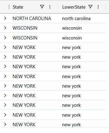
And, finally, let’s lowercase all the names by using KQL:

//select and rename columns
Weather
| project State
          , LowerState = tolower(State)

Conditional column

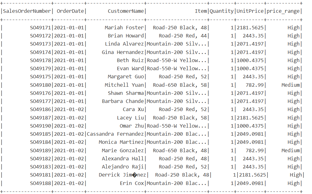
• PySpark – in the following example, we are creating a conditional column price_range, based on the value in the existing UnitPrice column. If the value is greater than 1000, we want to set the value of the price_range to “High”. If it’s greater than 500, then the price_range is “Medium”. For all the other values, the price_range will return “Low”. You might be thinking: wait, if there is a Unit Price value of, let’s say, 2000, this can be both High and Medium. However, the expression evaluation happens in the order you defined in the statement. First, it will check if the particular value is greater than 1000. If this evaluates to true, no further checks will be performed.

from pyspark.sql.functions import col, when

df = df.withColumn(
    "price_range",
    when(col("UnitPrice") > 1000, "High")
    .when(col("UnitPrice") > 500, "Medium")
    .otherwise("Low")
)
df.select("SalesOrderNumber","OrderDate","CustomerName","Item","Quantity","UnitPrice", "price_range").show()

• T-SQL

--Conditional column
SELECT SalesOrderNumber
    , OrderDate
    , CustomerName
    , Item
    , Quantity
    , UnitPrice
    , CASE 
        WHEN UnitPrice > 1000 THEN 'High'
        WHEN UnitPrice > 500 THEN 'Medium'
        ELSE 'Low'
    END AS PriceRange
FROM dbo.orders

• KQL

//conditional column
Weather
| extend DamagePropertyClass = case (
    DamageProperty > 49999, "High"
    , DamageProperty > 9999, "Medium"
    , "Low"
)

Pivot transformation

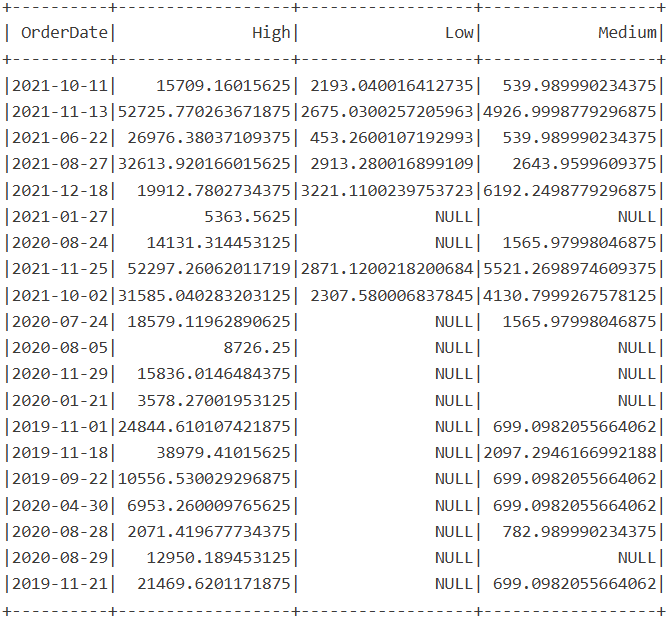
Sometimes, we need to tweak the structure of the underlying data. Pivot transformation is a common example of transforming rows into columns. In this case, I’m creating a new dataframe df_pivot, which first groups the data by the order date, then pivots values from the price_range column, remember those highs, mediums, and lows from the previous example, and calculates the sum of the unit price.

df_pivot = df.groupBy("OrderDate").pivot("price_range").sum("UnitPrice")

df_pivot.show()

The T-SQL implementation requires slightly more complex code, as you may notice in the following snippet:

--PIVOT Transformation
SELECT 
    OrderDate 
    , [High] 
    , [Medium] 
    , [Low] 
FROM (
    SELECT 
        OrderDate
        , UnitPrice
        , CASE 
        WHEN UnitPrice > 1000 THEN 'High'
        WHEN UnitPrice > 500 THEN 'Medium'
        ELSE 'Low'
    END AS PriceRange
    FROM dbo.orders
) AS SourceTable
PIVOT (
    SUM(UnitPrice)
    FOR PriceRange IN ([High], [Medium], [Low])
) AS PivotTable;

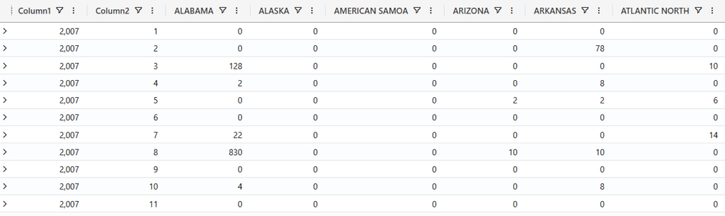
Unlike PySpark and T-SQL, which both provide a built-in pivot function, there is no such function in KQL. However, there is a pivot plugin, and we can mimic PIVOT behavior by combining the summarize and evaluate operators. In this example, we are summing injuries direct per year, month and state, and then pivoting states to be columns.

//Pivot transformation
Weather
| summarize Total = sum(InjuriesDirect) by datetime_part ("year", StartTime), datetime_part ("month", StartTime), State
| evaluate pivot(State, sum(Total))

Aggregation and grouping

Let’s wrap it up by examining how to perform aggregation and grouping operations when transforming the data. This is one of the most frequent requirements in analytical scenarios.

First, PySpark. I’m grouping the data by the year and month columns, and then I’m performing the sum aggregate function on the Unit price column. In the last step, we can also rename the column if needed, which I did here.

sales_by_yearMonth = orders_df.groupBy("Year", "Month").agg(
    {"UnitPrice": "sum"}
).withColumnRenamed("sum(UnitPrice)", "Unit_Price")

sales_by_yearMonth.show()

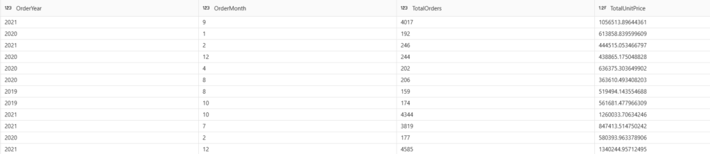
Now, T-SQL:

--Aggregate and group data
SELECT YEAR(OrderDate) as OrderYear
    , MONTH(OrderDate) as OrderMonth
    , count(*) as TotalOrders
    , SUM(UnitPrice) as TotalUnitPrice
FROM dbo.orders
GROUP BY YEAR(OrderDate)
    , MONTH(OrderDate)

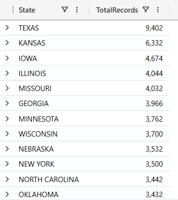
And, finally, KQL:

//aggregate and group data
//Use summarize operator
Weather
| summarize TotalRecords = count() by State

Conclusion

By understanding and leveraging the strengths of PySpark, T-SQL, and KQL, you can efficiently handle numerous data transformation tasks in Microsoft Fabric. Whether it’s filtering, aggregating, pivoting, cleaning, or enriching the data, choosing the right language for each scenario will enable faster and more resilient workflows, enhance productivity, and deliver more value from the raw data.

Thanks for reading!

Last Updated on May 27, 2025 by Nikola