Real-Time Intelligence in Microsoft Fabric - The Ultimate Guide!

Once upon a time, handling streaming data was considered an avanguard approach. Since the introduction of relational database management systems in the 1970s and traditional data warehousing systems in the late 1980s, all data workloads began and ended with the so-called batch processing. Batch processing relies on the concept of collecting numerous tasks in a group (or batch) and processing these tasks in a single operation.

On the flip side, there is a concept of streaming data. Although streaming data is still sometimes considered a cutting-edge technology, it already has a solid history. Everything started in 2002, when Stanford University researchers published the paper called “Models and Issues in Data Stream Systems”. However, it wasn’t until almost one decade later (2011) that streaming data systems started to reach a wider audience, when the Apache Kafka platform for storing and processing streaming data was open-sourced. The rest is history, as people say. Nowadays, processing streaming data is not considered a luxury, but a necessity.

This is the excerpt from the early release of the “Fundamentals of Microsoft Fabric” book, that I’m writing together with Ben Weissman (X) for O’Reilly. You can already read the early release, which is updated chapter by chapter, here.

Microsoft recognized the growing need to process the data “as soon as it arrives”. Hence, Microsoft Fabric doesn’t disappoint in that regard, as Real-time Intelligence is at the core of the entire platform and offers a whole range of capabilities to handle streaming data efficiently.

Before we dive deep into explaining each component of Real-time Intelligence, let’s take one step back and take a more tool-agnostic approach to stream processing in general.

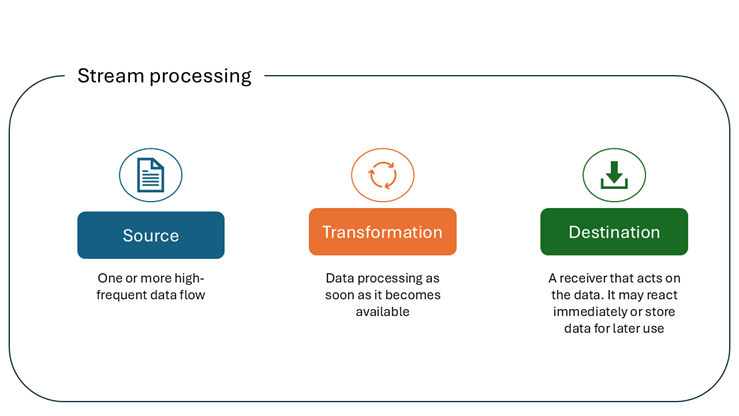
What is stream processing?

If you enter the phrase from the section title in Google Search, you’ll get more than 100,000 results! Therefore, we’re sharing an illustration that represents our understanding of stream processing.

Let’s now examine typical use cases for stream processing:

Fraud detection
Real-time stock trades
Customer activity
Log monitoring – troubleshooting systems, devices, etc.
Security information and event management – analyzing logs and real-time event data for monitoring and threat detection
Warehouse inventory
Ride share matching
Machine learning and predictive analytics

As you may have noticed, streaming data has become an integral part of numerous real-life scenarios and is considered vastly superior to traditional batch processing for the aforementioned use cases.

Let’s now explore how streaming data processing is performed in Microsoft Fabric and which tools of trade we have at our disposal.

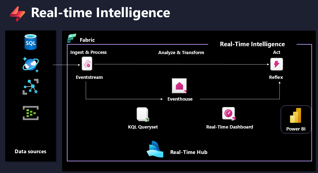
The following illustration shows the high-level overview of all Real-time Intelligence components in Microsoft Fabric:

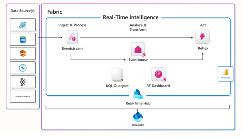
Real-Time hub

Let’s kick it off by introducing a Real-Time hub. Every Microsoft Fabric tenant automatically provisions a Real-Time hub. This is a focal point for all data-in-motion across the entire organization. Similar to OneLake, there can be one, and only one, Real-Time hub per tenant – this means, you can’t provision or create multiple Real-Time hubs.

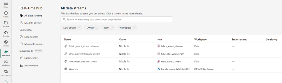
The main purpose of the Real-Time hub is to enable quick and easy discovery, ingestion, managing, and consuming streaming data from a wide range of sources. In the following illustration, you can find the overview of all the data streams in the Real-Time hub in Microsoft Fabric:

Let’s now explore all the available options in the Real-Time hub.

All data streams tab displays all the streams and tables you can access. Streams represent the output from Fabric eventstreams, whereas tables come from KQL databases. We will explore both evenstreams and KQL databases in more detail in the following sections
My data streams tab shows all the streams you brought into Microsoft Fabric into My workspace
Data sources tab is at the core of bringing the data into Fabric, both from inside and outside. Once you find yourself in the Data sources tab, you can choose between numerous, out-of-the-box provided connectors, such as Kafka, CDC streams for various database systems, external cloud solutions like AWS and GCP, and many more
Microsoft sources tab filters out the previous set of sources to include Microsoft data sources only
Fabric events tab displays the list of system events generated in Microsoft Fabric that you can access. Here, you may choose between Job events, OneLake events, and Workspace item events. Let’s dive into each of these three options:
- Job events are events produced by status changes on Fabric monitor activities, such as job created, succeeded, or failed
- OneLake events represent events produced by actions on files and folders in OneLake, such as file created, deleted, or renamed
- Workspace item events are produced by actions on workspace items, such as item created, deleted, or renamed
Azure events tab shows the list of system events generated in Azure blob storage

Real-Time hub provides various connectors for ingesting the data into Microsoft Fabric. It also enables creating streams for all of the supported sources. After the stream is created, you can process, analyze, and act on them.

Processing a stream allows you to apply numerous transformations, such as aggregate, filter, union, and many more. The goal is to transform the data before you send the output to supported destinations
Analyzing a stream enables you to add a KQL database as a destination of the stream, and then open the KQL Database and execute queries against the database.
Acting on streams assumes setting the alerts based on conditions and specifying actions to be taken when certain conditions are met

Eventstreams

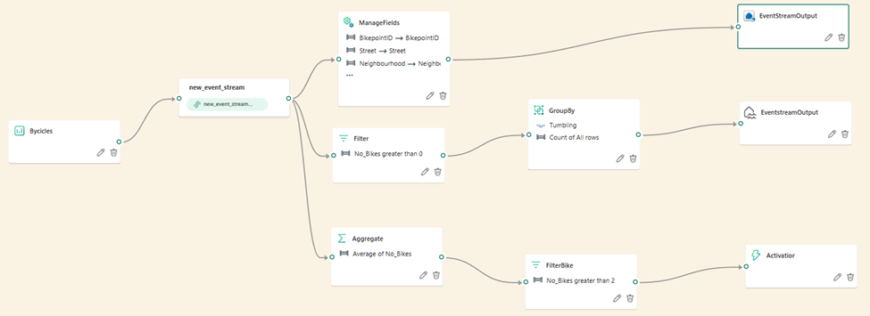
If you’re a low-code or no-code data professional and you need to handle streaming data, you’ll love Eventstreams. In a nutshell, Eventstream allows you to connect to numerous data sources, which we examined in the previous section, optionally apply various data transformation steps, and finally output results into one or more destinations. The following figure illustrates a common workflow for ingesting streaming data into three different destinations – Eventhouse, Lakehouse, and Activator:

Within the Eventstream settings, you can adjust the retention period for the incoming data. By default, the data is retained for one day, and events are automatically removed when the retention period expires.

Aside from that, you may also want to fine-tune the event throughput for incoming and outgoing events. There are three options to choose from:

Low: < 10 MB/s
Medium: 10-100 MB/s
High: > 100 MB/s

Eventhouse and KQL database

In the previous section, you’ve learned how to connect to various streaming data sources, optionally transform the data, and finally load it into the final destination. As you might have noticed, one of the available destinations is the Eventhouse. In this section, we’ll explore Microsoft Fabric items used to store the data within the Real-Time Intelligence workload.

Eventhouse

We’ll first introduce the Eventhouse item. The Eventhouse is nothing else but a container for KQL databases. Eventhouse itself does not store any data – it simply provides the infrastructure within the Fabric workspace for dealing with streaming data. The following figure displays the System overview page of the Eventhouse:

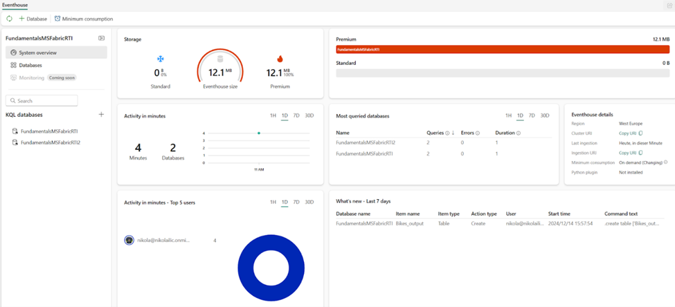
The great thing about the System overview page is that it provides all the key information at a glance. Hence, you can immediately understand the running state of the eventhouse, OneLake storage usage, further broken down per individual KQL database level, compute usage, most active databases and users, and recent events.

If we switch to the Databases page, we will be able to see a high-level overview of KQL databases that are part of the existing Eventhouse, as shown in below:

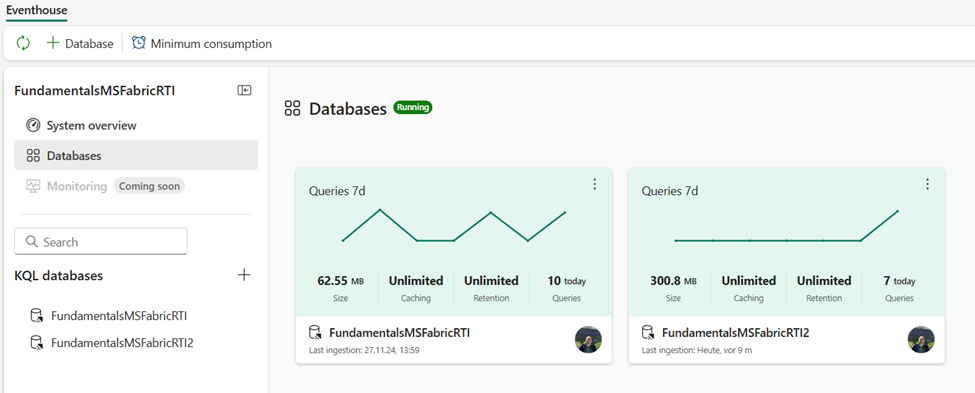
You can create multiple eventhouses in a single Fabric workspace. Also, a single eventhouse may contain one or more KQL databases:

Let’s wrap up the story about the Eventhouse by explaining the concept of Minimum consumption. By design, the Eventhouse is optimized to auto-suspend services when not in use. Therefore, when these services are reactivated, it might take some time for the Eventhouse to be fully available again. However, there are certain business scenarios when this latency is not acceptable. In those scenarios, make sure to configure the Minimum consumption feature. By configuring the Minimum consumption, the service is always available, but you are in charge of determining the minimum level, which is then available for KQL databases inside the Eventhouse.

KQL database

Now that you’ve learned about the Eventhouse container, let’s focus on examining the core item for storing real-time analytics data – the KQL database.

Let’s take one step back and explain the name of the item first. While most data professionals have at least heard about SQL (which stands for Structured Query Language), we are quite confident that KQL is way more cryptic than its “structured” relative.

You might have rightly assumed that QL in the abbreviation stands for Query Language. But, what does this letter K represent? It’s an abbreviation for Kusto. We hear you, we hear you: what is now Kusto?! Although the urban legend says that the language was named after the famous polymath and oceanographer Jacques Custeau (his last name is pronounced “Kusto”), we couldn’t find any official confirmation from Microsoft to confirm this story. What is definitely known is that it was the internal project name for the Log Analytics Query Language.

When we talk about history, let’s share some more history lessons. If you ever worked with Azure Data Explorer (ADX) in the past, you are in luck. KQL database in Microsoft Fabric is the official successor of ADX. Similar to many other Azure data services that were rebuilt and integrated into SaaS-fied nature of Fabric, ADX provided platform for storing and querying real-time analytics data for KQL databases. The engine and core capabilities of the KQL database are the same as in Azure Data Explorer – the key difference is the management behavior: Azure Data Explorer represents a PaaS (Platform-as-a-Service), whereas KQL database is a SaaS (Software-as-a-Service) solution.

Although you may store any data in the KQL database (non-structured, semi-structured, and structured), its main purpose is handling telemetry, logs, events, traces, and time series data. Under the hood, the engine leverages optimized storage formats, automatic indexing and partitioning, and advanced data statistics for efficient query planning.

Let’s now examine how to leverage the KQL database in Microsoft Fabric to store and query real-time analytics data. Creating a database is as straightforward as it could be. The following figure illustrates the 2-step process of creating a KQL database in Fabric:

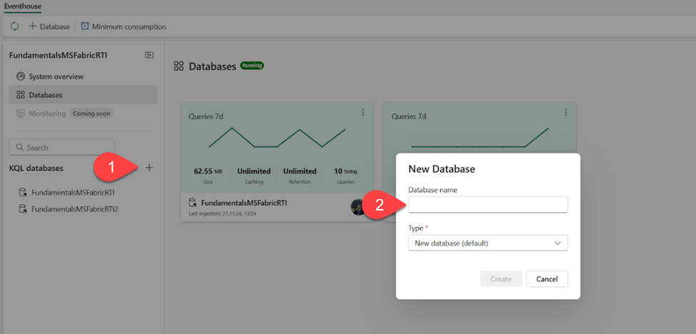
Click on the “+” sign next to KQL databases
Provide the database name and choose its type. Type can be the default new database, or a shortcut database. Shortcut database is a reference to a different database that can be either another KQL database in Real-Time Intelligence in Microsoft Fabric, or an Azure Data Explorer database

Don’t mix the concept of OneLake shortcuts with the concept of shortcut database type in Real-Time Intelligence! While the latter simply references the entire KQL/Azure Data Explorer database, OneLake shortcuts allow the use of the data stored in Delta tables across other OneLake workloads, such as lakehouses and/or warehouses, or even external data sources (ADLS Gen2, Amazon S3, Dataverse, Google Cloud Storage, to name a few). This data can then be accessed from KQL databases by using the external_table() function

Let’s now take a quick tour of the key features of the KQL database from the user-interface perspective. The figure below illustrates the main points of interest:

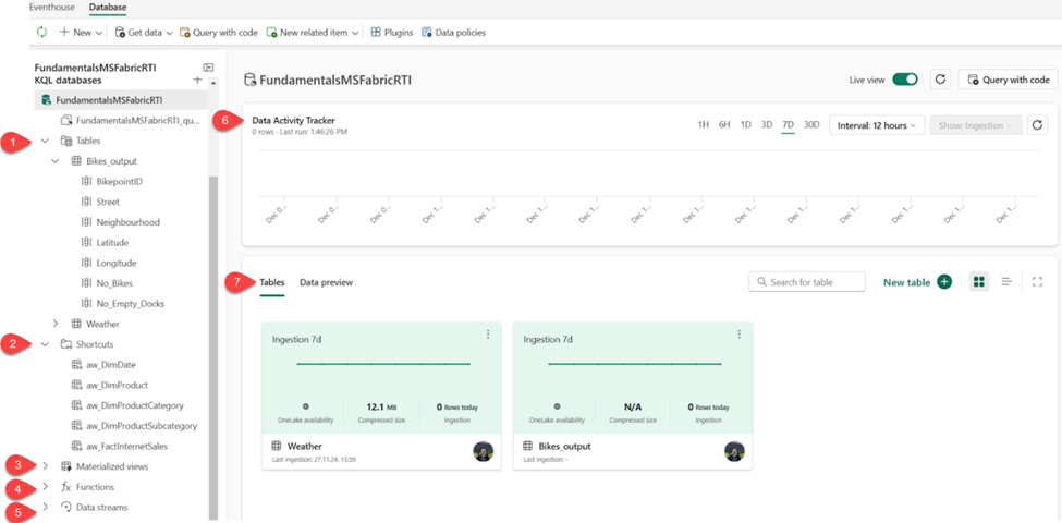
Tables – displays all the tables in the database
Shortcuts – shows tables created as OneLake shortcuts
Materialized views – a materialized view represents the aggregation query over a source table or another materialized view. It consists of a single summarize statement
Functions – these are User-defined functions stored and managed on a database level, similar to tables. These functions are created by using the .create function command
Data streams – all streams that are relevant for the selected KQL database
Data Activity Tracker – shows the activity in the database for the selected time period
Tables/Data preview – enables switching between two different views. Tables displays the high-level overview of the database tables, whereas Data preview shows the top 100 records of the selected table

Query and visualize data in Real-Time Intelligence

Now that you’ve learned how to store real-time analytics data in Microsoft Fabric, it’s time to get our hands dirty and provide some business insight out of this data. In this section, we will focus on explaining various options for extracting useful information from the data stored in the KQL database.

Hence, in this section, we will introduce common KQL functions for data retrieval, and explore Real-time dashboards for visualizing the data.

KQL queryset

The KQL queryset is the fabric item used to run queries and view and customize results from various data sources. As soon as you create a new KQL database, the KQL queryset item will be provisioned out of the box. This is a default KQL queryset that is automatically connected to the KQL database under which it exists. The default KQL queryset doesn’t allow multiple connections.

On the flip side, when you create a custom KQL queryset item, you can connect it to multiple data sources, as shown in the following illustration:

Let’s now introduce the building blocks of the KQL and examine some of the most commonly used operators and functions. KQL is a fairly simple yet powerful language. To some extent, it’s very similar to SQL, especially in terms of using schema entities that are organized in hierarchies, such as databases, tables, and columns.

The most common type of KQL query statement is a tabular expression statement. This means that both query input and output consist of tables or tabular datasets. Operators in a tabular statement are sequenced by the “|” (pipe) symbol. Data is flowing (is piped) from one operator to the next, as displayed in the following code snippet:

MyTable

| where StartTime between (datetime(2024-11-01) .. datetime(2024-12-01))

| where State == "Texas"  

| count

The piping is sequential – the data is flowing from one operator to another – this means that the query operator order is important and may have an impact on both the output results and performance.

In the above code example, the data in MyTable is first filtered on the StartTime column, then filtered on the State column, and finally, the query returns a table containing a single column and single row, displaying the count of the filtered rows.

The fair question at this point would be: what if I already know SQL? Do I need to learn another language just for the sake of querying real-time analytics data? The answer is as usual: it depends.

Luckily, we have good and great news to share here!

The good news is: you CAN write SQL statements to query the data stored in the KQL database. But, the fact that you can do something, doesn’t mean you should…By using SQL-only queries, you are missing the point, and limitting yourself from using many KQL-specific functions that are built to cope with real-time analytics queries in the most efficient way

The great news is: by leveraging the explain operator, you can “ask” Kusto to translate your SQL statement into an equivalent KQL statement, as displayed in the following figure:

In the following examples, we will query the sample Weather dataset, which contains data about weather storms and damages in the USA. Let’s start simple and then introduce some more complex queries. In the first example, we will count the number of records in the Weather table:

//Count records
Weather
| count

Wondering how to retrieve only a subset of records? You can use either take or limit operator:

//Sample data
Weather
| take 10

Please keep in mind that the take operator will not return the TOP n number of records, unless your data is sorted in the specific order. Normally, the take operator returns any n number of records from the table.

In the next step, we want to extend this query and return not only a subset of rows, but also a subset of columns:

//Sample data from a subset of columns
Weather
| take 10
| project State, EventType, DamageProperty

The project operator is the equivalent of the SELECT statement in SQL. It specifies which columns should be included in the result set.

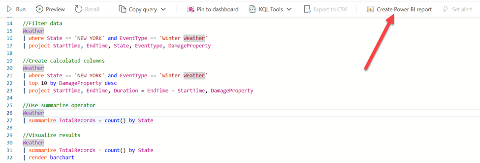
In the following example, we are creating a calculated column, Duration, that represents a duration between EndTime and StartTime values. In addition, we want to display only top 10 records sorted by the DamageProperty value in descending order:

//Create calculated columns
Weather
| where State == 'NEW YORK' and EventType == 'Winter Weather'
| top 10 by DamageProperty desc
| project StartTime, EndTime, Duration = EndTime - StartTime, DamageProperty

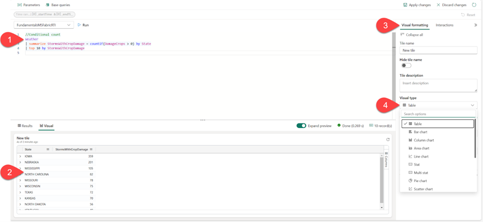
It’s the right moment to introduce the summarize operator. This operator produces a table that aggregates the content of the input table. Hence, the following statement will display the total number of records per each state, including only the top 5 states:

//Use summarize operator
Weather
| summarize TotalRecords = count() by State
| top 5 by TotalRecords

Let’s expand on the previous code and visualize the data directly in the result set. I’ll add another line of KQL code to render results as a bar chart:

As you may notice, the chart can be additionally customized from the Visual formatting pane on the right-hand side, which provides even more flexibility when visualizing the data stored in the KQL database.

These were just basic examples of using KQL language to retrieve the data stored in the Eventhouse and KQL databases. We can assure you that KQL won’t let you down in more advanced use cases when you need to manipulate and retrieve real-time analytics data.

We understand that SQL is the “Lingua franca” of many data professionals. And although you can write SQL to retrieve the data from the KQL database, we strongly encourage you to refrain from doing this. As a quick reference, we are providing you with a “SQL to KQL cheat sheet” to give you a head start when transitioning from SQL to KQL.

Also, my friend and fellow MVP Brian Bønk published and maintains a fantastic reference guide for the KQL language here. Make sure to give it a try if you are working with KQL.

Real-time dashboards

While KQL querysets represent a powerful way of exploring and querying data stored in Eventhouses and KQL databases, their visualization capabilities are pretty limited. Yes, you can visualize results in the query view, as you’ve seen in one of the previous examples, but this is more of a “first aid” visualization that won’t make your managers and business decision-makers happy.

Fortunately, there is an out-of-the-box solution in Real-Time Intelligence that supports advanced data visualization concepts and features. Real-Time Dashboard is a Fabric item that enables the creation of interactive and visually appealing business-reporting solutions.

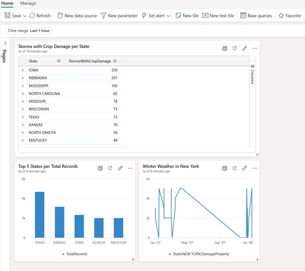
Let’s first identify the core elements of the Real-Time Dashboard. A dashboard consists of one or more tiles, optionally structured and organized in pages, where each tile is populated by the underlying KQL query.

As a first step in the process of creating Real-Time Dashboards, this setting must be enabled in the Admin portal of your Fabric tenant:

Next, you should create a new Real-Time Dashboard item in the Fabric workspace. From there, let’s connect to our Weather dataset and configure our first dashboard tile. We’ll execute one of the queries from the previous section to retrieve the top 10 states with the conditional count function. The figure below shows the tile settings panel with numerous options to configure:

KQL query to populate the tile
Visual representation of the data
Visual formatting pane with options to set the tile name and description
Visual type drop-down menu to select the desired visual type (in our case, it’s table visual)

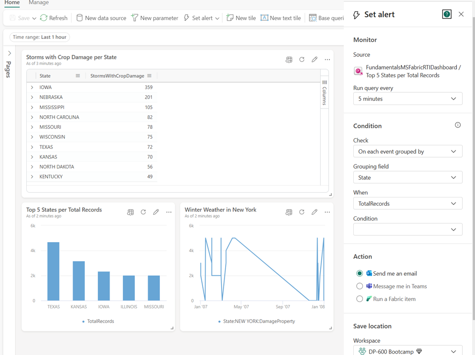
Let’s now add two more tiles to our dashboard. I’ll copy and paste two queries that we previously used – the first will retrieve the top 5 states per total number of records, whereas the other will display the damage property value change over time for the state of New York and for event type, which equals winter weather.

You can also add a tile directly from the KQL queryset to the existing dashboard, as illustrated below:

Let’s now focus on the various capabilities you have when working with Real-Time Dashboards. In the top ribbon, you’ll find options to add a New data source, set a new parameter, and add base queries. However, what really makes Real-Time Dashboards powerful is the possibility to set alerts on a Real-Time Dashboard. Depending if the conditions defined in the alert are met, you can trigger a specific action, such as sending an email or Microsoft Teams message. An alert is created using the Activator item.

Visualize data with Power BI

Power BI is a mature and widely adopted tool for building robust, scalable, and interactive business reporting solutions. In this section, we specifically focus on examining how Power BI works in synergy with the Real-Time Intelligence workload in Microsoft Fabric.

Creating a Power BI report based on the data stored in the KQL database couldn’t be easier. You can choose to create a Power BI report directly from the KQL queryset, as displayed below:

Each query in the KQL queryset represents a table in the Power BI semantic model. From here, you can build visualizations and leverage all the existing Power BI features to design an effective, visually appealing report.

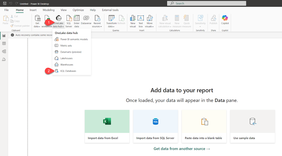
Obviously, you can still leverage the “regular” Power BI workflow, which assumes connecting from the Power BI Desktop to a KQL database as a data source. In this case, you need to open a OneLake data hub and select KQL Databases as a data source:

The same as for SQL-based data sources, you can choose between the Import and DirectQuery storage modes for your real-time analytics data. Import mode creates a local copy of the data in Power BI’s database, whereas DirectQuery enables querying the KQL database in near-real-time.

Activator

Activator is one of the most innovative features in the entire Microsoft Fabric realm. I’ll cover Activator in detail in a separate article. Here, we just want to introduce this service and briefly emphasize its main characteristics.

Activator is a no-code solution for automatically taking actions when conditions in the underlying data are met. Activator can be used in conjunction with Eventstreams, Real-Time Dashboards, and Power BI reports. Once the data hits a certain threshold, the Activator automatically triggers the specified action – for example, sending the email or Microsoft Teams message, or even firing Power Automate flows. I’ll cover all these scenarios in more depth in a separate article, where I also provide some practical scenarios for implementing the Activator item.

Conclusion

Real-Time Intelligence – something that started as a part of the “Synapse experience” in Microsoft Fabric, is now a separate, dedicated workload. That tells us a lot about Microsoft’s vision and roadmap for Real-Time Intelligence!

Don’t forget: initially, Real-Time Analytics was included under the Synapse umbrella, together with Data Engineering, Data Warehousing, and Data Science experiences. However, Microsoft thought that handling streaming data deserves a dedicated workload in Microsoft Fabric, which absolutely makes sense considering the growing need to deal with data in motion and provide insight from this data as soon as it is captured. In that sense, Microsoft Fabric provides a whole suite of powerful services, as the next generation of tools for processing, analyzing, and acting on data as it’s generated.

We are quite confident that the Real-Time Intelligence workload will become more and more significant in the future, considering the evolution of data sources and the increasing pace of data generation.

Thanks for reading!