Partitioning is one of the key concepts when you work with big data. When I say big, I mean really BIG! Obviously, if you deal with few millions or even tens of millions records, partition will bring more overhead than benefit and you should think twice before implementing it.
Horizontal vs Vertical partitioning
First of all, there are two ways of partitioning – horizontal and vertical. Horizontal partitioning (or row-based partitioning) means that data is split in multiple tables based on predicate you define (most often it relates to dates, so data is being partitioned by year, month, even day – if it makes sense in your scenario). Of course, data can be partitioned based on other criteria – for example, users with last names starting from A – M in one table, users with last names starting from N – Z in other. Key takeaway here is that data is being stored in separate tables.
On the other side, vertical partitioning (or column-based partitioning) is being performed when you have too “wide” table with many columns, which can be moved to other tables using normalization. Imagine that you have huge fact table with billions of rows, structured like in the following picture:
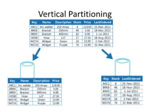
It consumes a hell of a lot of memory, so you can normalize the table and move some attributes to the other table.
SSAS Partitioning
Comparing to database partitioning methods mentioned above, I would say that SSAS Cube partitioning doesn’t share many things in common, except sharing name of course:)
So, what is partitioning within SSAS Cube? Basically, concept is the same, you break data into smaller chunks, usually based on time dimension (year, quarter, month…). But, while partitioning in relational databases’ world are done using only one type of segmentation (let’s say per month), in SSAS you can create partitions based on different level of granularity. That said, you can create partitions on year level for older data, and on month level for recent data. Additionally, aggregations can also be different within different partitions.
By default, when you create a Cube, all of your figures resides in one big partition called Measure Group.
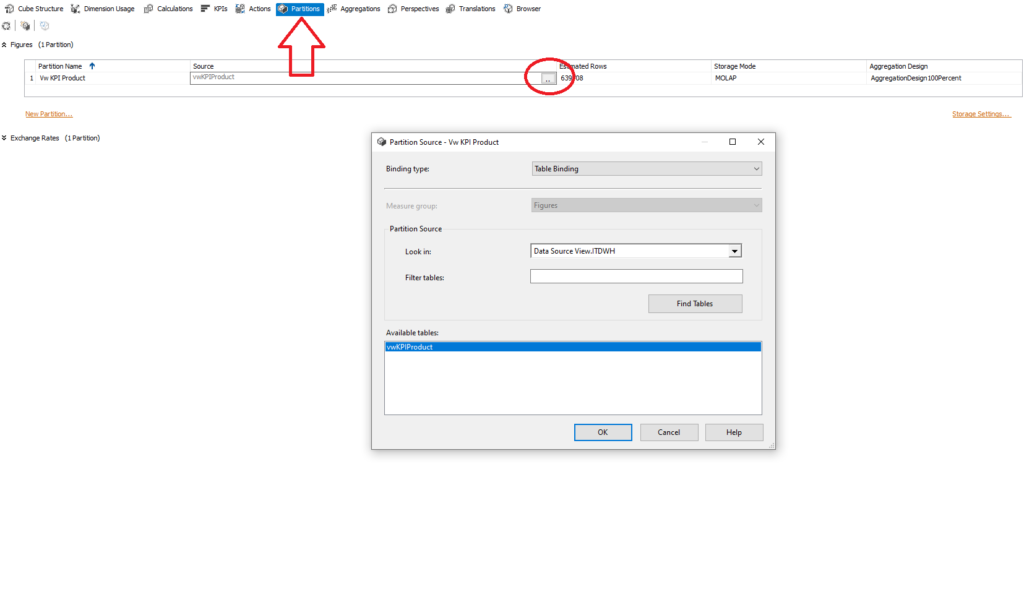
In order to create separate partitions, you need to switch from Table Binding to Query Binding under Partition tab of the Cube.
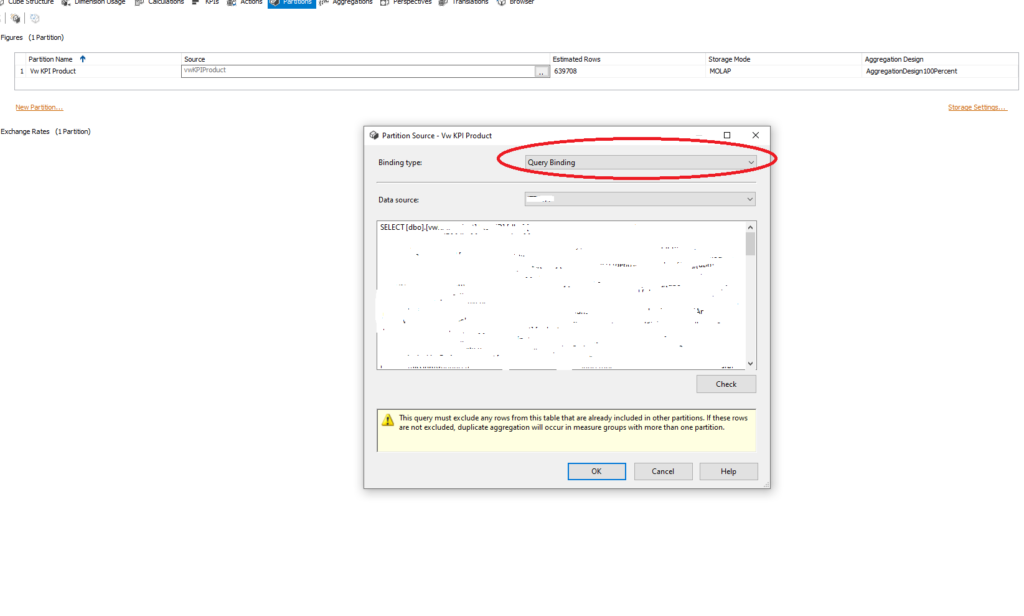
From there, you create regular SQL query which will generate subset of data for that partition.
Processing cube partitions
Partitioning data can have huge impact on cube processing, because you can process different partitions using different processing methods. That being said, processing one large (default) partition can be quite slow and CPU exhausting. With different partitions, you can spread processing to best suit your needs.
For example, partitions which contain older data, for which you are sure that won’t be changed, you can use, let’s say, Process Default, while for more recent data you can choose another processing type. Just make sure that your partitions don’t overlap, since you will have duplicates once the cube is processed.
More about processing types can be found here. I strongly recommend reading this article carefully and try to find best possible processing types for your scenario. In my case, with performing Process Update on my dimensions and Process Default on partitions, I managed to reduce total processing time significantly (up to 5 times faster).
Last Updated on February 24, 2020 by Nikola